When predicting readmission for hospitalized people with diabetes, comparisons that maintain patient independence must be made and that separate from the discrimination of the risk estimates are their reliability and practical implications. Objective: Traditional vs. ensemble classifiers for recorded readmission within 30 days of discharge and the contribution of feature families. The UCI Diabetes 130-US Hospitals dataset was restricted to eligible discharges, which included 98,470 encounters from 69,305 patients, aged 20 years or older. Patients were divided into different training, calibration, threshold selection, and test partitions. The same three-fold grouped cross validation was performed for nine classifiers with three sampled hyperparameter configurations for each model. AP (average precision) was used to select models. In each partition, a policy of sigmoid calibration and a 80% sensitivity threshold was fitted. The evaluation consisted of 500 patient-cluster bootstrap replicates, 12 ablations, subgroup checks, decision curves, and sampled SHAP explanations. Results: Cross-validation was used to select the histogram gradient boosting. On 19,693 test encounters, AP was 0.2258 (95% interval 0.2034–0.2553), AUROC was 0.6704, and the Brier score was 0.0966. Its paired AP advantage over logistic regression was 0.0180 (95% interval 0.0118–0.0252). The sensitivity, specificity, and precision of the locked threshold were 79.88%, 42.14%, and 15.13%, respectively. The AP dropped to 0.1894 when prior utilization was removed and to 0.1994 when administrative features were removed. The test AP for the secondary soft-voting ensemble was the highest observed at 0.2269 but was not used to replace the model that was previously selected before testing. Conclusion: Ensemble methods provided marginal improvement on patient-separated evaluation. But previous use and administrative knowledge were strong factors, and historical data constraints and a high false-positive burden make it impossible to say how ready the clinical use is.
Research ArticleClinical Machine LearningIn progress
A Comparative Study of Machine Learning Algorithms for Early Disease Prediction Using Public Healthcare Datasets
Correspondence: tresnadey98@gmail.com
Abstract
Keywords diabeteshospital readmissioncomparative machine learningpatient-grouped validationprobability calibrationSHAP
1 Introduction
A prognostic outcome is hospital readmission, which can be used to identify patients who might require further assistance after they leave the hospital. Review of validated readmission models revealed differences in predictive performance and generalizability based on the population and purpose of the model with limited representation of functional and social data [1]. It is therefore reasonable to employ diabetes-specific risk assessment for comparative prediction research. The Diabetes Early Readmission Risk Indicator has shown that routine clinical and sociodemographic information can be used for a viable risk model but still leave significant unexplained variation [2]. The choice of definition of an outcome in public datasets affects the kinds of questions that can be addressed, and model comparisons can be reproducible.
The UCI Diabetes 130-US Hospitals dataset provides hospital encounters where diabetes is documented but does not track patients of a disease-free population to the onset of diabetes [3]. The source study included an analysis of the relationship between measurement of HbA1c and readmission [4]. The present study therefore aims to predict the readmission post-discharge in patients with diabetes. It is not intended to predict the onset of diabetes or an admission time screening tool. It's not just about the highest accuracy reported for an algorithm. One general readmission comparison identified that flexible methods might be more effective in certain cases [5], while a more comprehensive survey of all clinical prediction studies did not reveal overall superior performance of machine learning over logistic regression [6].
The model rankings are influenced by the cohort, availability of predictors, validation design, tuning budget, and evaluation metric used. These are particularly applicable when there are multiple encounters for the same patient and the positive result is rare. This paper compares the performance of nine classifiers, both traditional and ensemble, in a standard discharge-time prediction pipeline. It separates model development, probability calibration, threshold selection, and final evaluation per patient. The contribution is a transparent comparison under this specified protocol, in conjunction with patient-cluster uncertainty intervals and ablations that assess the impact of information availability. The algorithms are nothing new, nor is the combination of algorithms and SHAP.
1.1 Objectives and research questions
The goals are to compare the predictive performances under a common patient-separated design, quantify the operational consequences of adopting a threshold based on the sensitivity to the model, and determine which families of features support the selected model. Three questions are asked in the analysis: RQ1: Which model has the best training cross-validation AP, and what is the difference between its AP and logistic regression on unseen patients? RQ2: What is the resulting performance difference of feature removal, training sample size, class weighting, repeated encounters, and calibration? RQ3: What do calibration, subgroup evaluation, and model explanation tell us about the utility and limitations of the resulting predictions?
2 Literature Review
2.1 Readmission models in patients with diabetes
The source analysis of the UCI records involved multivariable logistic regression analysis of HbA1c measurement and early readmission, and the effect varied by primary diagnosis [4]. This focus on associations with care processes is not an algorithm comparison. A second clinical population was studied in the DERRI development study, where 44,203 discharges were analyzed, and the validation C statistic was 0.69 [2]. The C statistic obtained from external validation was next 0.634, based on 105,974 discharges, indicating that the performance can vary by a substantial amount in a different population [7]. These studies lend to an interpretable regression comparator and caution for transportability. A number of studies have been conducted on this UCI data comparing different machine learning algorithms.
An analysis of 100,244 records with 23 attributes, from 2021, retained the prior hospital use as one of the influential predictors and compared random forest, naïve Bayes, and tree ensembles [8]. In 2024, a study was done comparing ten conventional classifiers with a neural sequence model with feature selection using the Grey Wolf Optimizer, group cross validation, and synthetic minority oversampling [9]. Another work was based on genetic-algorithm tuning and support vector machine, where classification accuracy was reported along with other threshold-dependent metrics [10]. These papers point towards the fact that the comparative modelling and ensemble evaluation have already been explored on this data set. Some more recent papers also have methodological aspects that are sometimes introduced as new.
Logistic regression, random forest, XGBoost, LightGBM, and stacking, along with nested cross-validation, probability calibration, bootstrap evaluation, decision curves, and SHAP, were included in the 2026 study of the UCI cohort. It achieved a stacking AUROC of 0.664 in nested cross validation and 0.688 in its calibrated analysis [11]. This means that the presence of calibration, explainability, or an ensemble alone does not constitute a new research contribution. An effective extension should clearly describe what decisions of evaluation and empirical questions have changed.
2.2 Validation and evaluation requirements
The methodological research discusses the significance of these differences. Reusing the cross-validation results for tuning and final performance estimation may lead to the selection optimism [12]. Based on the structured observations, it is also revealed that validation should represent the relationship of dependence between records [13]. A survey of leakage in machine learning research shows how wrong information can lead to wrong conclusions [14]. The appropriate separation unit for the present generalization question should be the patient, not an individual row, since the patient has frequent contacts with the person. This doesn't mean separation by hospital or calendar time. Another place where there appears to be disagreement is in the choice of metric.
Precision–recall evaluation emphasizes the focus of true events in positive predictions for imbalanced data, whereas ROC analysis examines the sensitivity–specificity range of discrimination [15], [16]. Calibration evaluates the extent to which the estimated probabilities match the observed frequencies and cannot be used without AUROC. A general performance rating system calls for the assessment of discrimination and calibration and decision analysis if it is desired to use the forecasts to inform action [18]. Under the explicit threshold interpretation, a tradeoff between correctly identifying events and unnecessary intervention can be expressed in decision curves [19]. The definition of the participants, predictors, outcomes, and evaluation procedures are also central to current reporting and appraisal guidance [20], [21].
These sources inspire a protocol that is endpoint-oriented, that is prediction-time-oriented, that requires no test outcomes to set thresholds, and that honors patient clustering in uncertainty. Reporting is done based on the above and not through the presumption of a formal independent TRIPOD+AI or PROBAST+AI assessment being undertaken.
2.3 Research gap and study contribution
The need for a tightly-scaled, auditable comparison that incorporates a stable, clinically defined endpoint with a stated separation policy at the patient level and an operating threshold is addressed here. The literature analyzed and reviewed already comprises grouped validation and extensive calibration/explainability analyses, and this paper is not the first to apply such analyses to this data. Its empirical analysis is the simultaneous analysis of feature-family ablations, training-data reductions, equal-patient evaluation, and prediction errors at an independently selected sensitivity target. These analyses assess if the chosen model is primarily diabetes-specific or primarily utilization/discharge data.
3 Methodology
3.1 Study design and outcome
We performed a retrospective comparative prediction study based on the publicly available dataset UCI Diabetes 130-US Hospitals and the associated administrative-code mapping file [3]. These source records cover the years 1999–2008 and pertain to inpatients who had been diagnosed with diabetes, had a hospital stay of 1–14 days, and had laboratory results and medication administered in the facility. The given file has 101,766 encounters, 71,518 different patient identifiers, and 50 columns. Encounters are the prediction units, and patients define partitions and bootstrap clusters. The positive outcome was "readmitted <30," and the negative outcome was "readmitted >30" or "readmitted NO." A conventional short label for less than 30 days is used here.
“NO” does not mean the absence of readmission was verified at all hospitals; rather, it means that no readmission was recorded in the source. It is not possible to reliably distinguish planned from unplanned admissions or preventable from nonpreventable events using the public files. They also don't have the event dates necessary for event reconstruction and examining censoring directly. We chose to include length of stay, completed encounter diagnoses, medication changes, and disposition during discharge, therefore making prediction possible at discharge. This is a complete feature-set that cannot be legitimately used by an admission-time model. The planned statistical objective was a new encounter with a different patient in the same data source as the prior encounter.
Hospital-level transportability and temporal transportability were not supported by the design, as membership at hospitals and event timestamps were not available in the released files.
3.2 Eligibility and patient allocation
Age bands were kept starting at 20 years and the bands below 20 years were excluded. This results in a population aged 20 years and older but should not be referred to as adults aged 18 years and older, since the 10-year age intervals are unable to capture ages 18-19. We excluded discharges coded 11, 19, 20, or 21 for death; 13 or 14 for hospice; and 9 or 12 for encounters coded to a discharge status that was not a completed leave from inpatient care. Other dispositions (transfers, etc.) were not reallocated to the primary cohort. Home-related discharges coded 1, 6 and 8 were analyzed separately in a descriptive analysis. There were 69,305 patients with 11,260 positive encounters in the data, which was reduced for eligibility. Cohorts and partitions are given in Table 1. The other two encounters were repeated so that the discharge-level prediction task was maintained. No patient was recorded in more than one partition. Since there is no reliable chronology, no retained record is called the first admission.
Table 1. Cohort construction and patient-separated partitions.
| Stage or partition | Encounters | Patients | Events |
|---|---|---|---|
| Supplied dataset | 101,766 | 71,518 | 11,357 |
| Age ≥20 years | 100,914 | 70,840 | 11,314 |
| Eligible cohort | 98,470 | 69,305 | 11,260 |
| Training | 59,084 | 41,580 | 6,756 |
| Calibration | 9,848 | 6,919 | 1,126 |
| Threshold selection | 9,845 | 6,936 | 1,126 |
| Test | 19,693 | 13,870 | 2,252 |
The split performed by allocation resulted in about 60% of patients being allocated for model training, 10% for calibration, 10% for threshold selection, and 20% for the final test set. Fold 0 was used as the test partition, fold 2 as the calibration partition, fold 3 as the threshold partition, and folds 4-9 were used as the training partition. The seed used for the allocations is 20261007. Stratification was applied just to balance the pre-defined partitions using outcomes only. Three other patient-grouped folds were used within the training partition for model tuning. Fig. 1 illustrates the sequence and demonstrates that all test patients were excluded from any fitting decision.
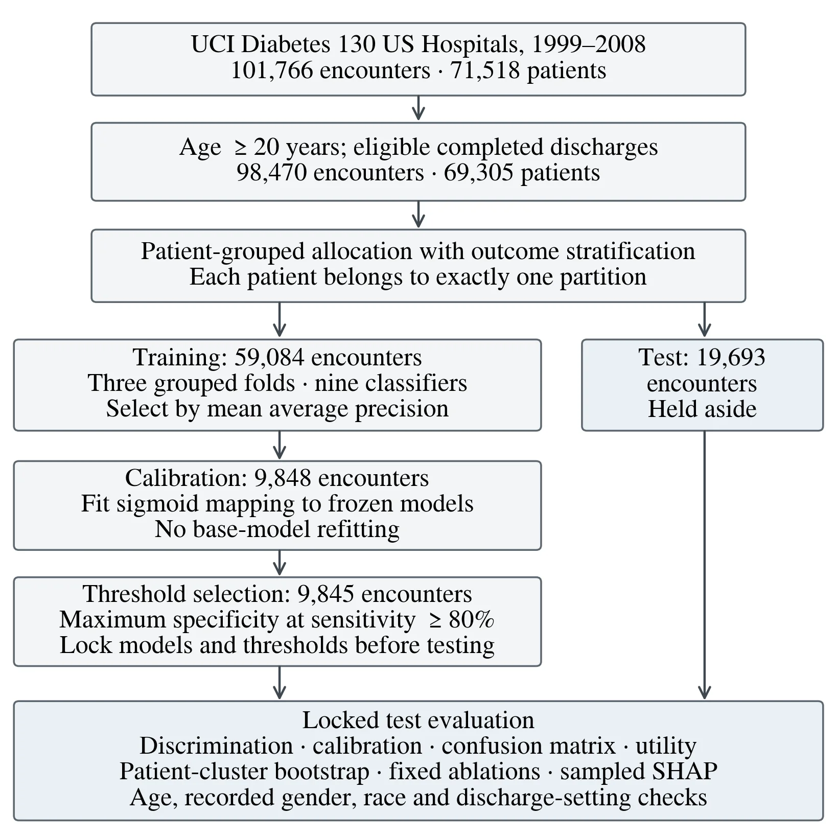
In Figure 1, the left branch is the three development stages, and the right branch is the held-out test partition. Calibration alters the mapping that transforms the scores into probabilities, without affecting the base classifier. The operating rule is then determined by the threshold selection. The branches are not together until the choices have been made and the branches evaluated. Ablations are also allocated in the same manner, and the updated options are not returned to the original model.
3.3 Feature construction and preprocessing
Identifiers were kept for auditing purposes and for grouping, but never for predictions. Weight and payer code were intentionally not included in this comparison due to significant missingness and inconsistent use for this comparison, whereas medical specialty was included with an explicit missing category. The missing value parsing parsed a “?” as missing but kept the actual lab value "None," which indicates that the test was not measured. Administrative codes that were not known or were not supplied were mapped to an unknown admin category. An encounter with “Unknown/Invalid” gender was not used to exclude an encounter but rather treated as missing.
The three diagnosis codes were coded to a higher level of aggregation, consisting of diabetes, circulatory, respiratory, digestive, genitourinary, injury, musculoskeletal, neoplasm, supplementary, external-cause, other, and missing categories from ICD-9. This helps decrease the sparsity of raw diagnosis codes and standardizes the input to the models. The seven prespecified feature families are listed in Table 2. The 45 original predictors are expanded after one-hot encoding, which is not the number of the regression coefficients that were fitted or the number of encoded columns.
Table 2. Predictor families in the full discharge-time model.
| Family | No. of fields | Included information |
|---|---|---|
| Prior utilization | 3 | Prior-year outpatient, emergency, and inpatient visit counts |
| Diagnosis | 4 | Three grouped ICD-9 diagnoses and total diagnosis count |
| Medication | 26 | Twenty-three medication-status fields, medication change, diabetes medication indicator, and medication count |
| Laboratory | 3 | HbA1c category, serum glucose category, and laboratory procedure count |
| Demographic | 3 | Age band, recorded gender, and recorded race |
| Administrative | 4 | Admission type, admission source, discharge disposition, and medical specialty |
| Stay intense. | 2 | Length of stay and number of procedures |
Table 2 distinguishes between information gained prior to and at the time of presentation and information gathered in the hospital. While prior utilization can provide a summary of all previous care encounters, discharge disposition and stay intensity would need the completed encounter. Medication fields were not interpreted as verified outpatient prescriptions and were considered as medication prescribed during the encounter. Demographic characteristics were as part of the full benchmark and in an ablation and subgroup analysis. All classifiers have applied the same preprocessing pipeline: median imputation, standardization of the numerical variables, explicit missing-category imputation, one-hot encoding of the categorical variables, and removal of the constant encoded variables. There were fewer than 20 examples in the training folds for some categories; these were grouped together, and unseen categories were handled by the fitted encoder. These transformations were only fitted within each training fold and then refitted on the full training fold for the chosen configuration. No feature selection, outcome-guided or test-based imputation, or synthetic oversampling was performed. Equal preprocessing is used to support a controlled comparison, but it might not result in maximum models that are able to deal with categorical or missing values natively.
3.4 Classifiers and model selection
Logistic regression, linear support vector machine, Gaussian naïve Bayes, and a decision tree were the traditional models. They offer additive, margin, probabilistic-independence, and single-tree comparators. The ensemble models used were Random Forest, Extra Trees, Histogram Gradient Boosting, XGBoost and LightGBM. The comparison includes the popular randomized tree aggregation and sequential boosting methods based on well-known algorithmic bases [22], [23], [24], [25], [26]. Logistic regression was kept as prespecified reference as extra model complexity must be warranted from the data. RandomizedSearchCV tested 3 samples of hyperparameter sets for each of the 3 different classifiers on the same 3 patient-grouped training sets. The best configuration and the primary model were obtained by mean validation AP.
Details of the finite search grids, sampled configurations, and fold scores are saved in the associated notebook. For tree ensembles, 160 trees (or boosting iterations) were used, and early stopping was turned off for the histogram gradient boosting. In primary models all the training observations were without weights. The equality in the number of searches does not mean equal computing cost or that all the models are optimized equally. Following the selection using train only, a soft voting with equal weights was used for three highest rated classifiers, namely histogram gradient boosting, XGBoost, and random forest that produce a probability. The members were retrained with the same training data, and the ensemble was still a secondary comparator.
A constant-prevalence predictor was used as a baseline. Thus, there is no directly comparable model-selection cross-validation score in the primary ranking for the vote and the prevalence baseline. The voting members or the selected model were not altered on the basis of final test results, nor was the search budget modified.
3.5 Calibration and operating threshold
The base estimator was frozen, and each fitted classifier, the secondary vote, and the prevalence baseline were sigmoid calibrated in the separate calibration partition. This will enable the probability quality to be compared following an identical calibration procedure, as different calibration methods are known to act differently over a range of model scores [27]. The fitted mapping for an underlying score sᵢ can be expressed as Equation (1). Only the calibration patients were used to estimate its coefficients A and B, and its score was either the decision function or the model probability.
p_i = 1 / (1 + exp(As_i + B)) (1)
The operating threshold was chosen on a third independent partition. The rule used a candidate threshold with the greatest specificity, among those that were observed, that satisfy the 0.80 sensitivity constraint and that break ties towards the largest threshold, as described in Equation (2). The sensitivity target is a rough guide to the policy for identifying a large risk group and is not based on a clinical cost study. This was the same rule for all classifiers, but the threshold value was different for each.
t* = arg max_t Specificity(t), subject to Sensitivity(t) ≥ 0.80 (2)
The test evaluation was then performed under the locked threshold. Not adjusted retroactively to achieve the target; sampling variation may cause test sensitivity to be less than or greater than 80%. A no-calibration ablation was performed with the selected model (not calibrated) and its threshold, which was also selected, on the same threshold partition.
3.6 Performance measures and uncertainty
Average precision was used as the primary metric, which can be calculated as the sum shown in Equation (3), with Pₖ and Rₖ being precision and recall at operating points ordered by increasing recall. AP is based on the positive outcome, and it uses the observed test prevalence as the constant-score reference. It is not the area under a precision–recall curve, which is trapezoidal. The secondary discrimination measure was the area under the receiver operating characteristic curve (AUROC). Brier score, log loss, sensitivity, specificity, precision, F1 score, balanced accuracy, Matthews correlation coefficient, and accuracy were also calculated. The emphasis in the primary article tables is on measures that are required to understand the ranking, the probability error, and the operating policy; the full outputs are stored in the notebook.
AP = ∑_{k = 1}^{K}(R_k − R_{k−1})P_k (3)
The Brier score in Equation (4) averages squared probability error over N test encounters. Lower values indicate better overall probabilistic accuracy, reflecting both discrimination and calibration. Calibration was also examined using eight quantile bins and a logistic calibration intercept and slope fitted solely for test-set assessment. Ideal values are zero and one, respectively. These diagnostic coefficients were not used to update the reported test predictions.
BS = 1 / N∑_{i = 1}^{N}(y_i − p_i)^2 (4)
500 percentile bootstrap replicates were used to estimate uncertainty, using test patients sampled with replacement, but keeping all the encounters for each sampled patient. This implements bootstrap resampling at the dependence unit level and does not assume independence between all rows [28]. Paired model differences were made using the same replicate samples. The main comparison was between the model picked by cross-validation and logistic regression in AP. Intervals are conditional on the fitted models and do not contain uncertainty related to repeating model training, hyperparameter selection, or partition allocation. Secondary comparisons and ablations are descriptive and are not adjusted for multiple testing. The primary estimand weights encounters equally. A sensitivity analysis, however, assigned each patient total weight according to the number of encounters in which they had a test by dividing 1 by the number of their encounters. This alters the population weighting and its event prevalence, and the resulting AP should not be interpreted as directly exchangeable with the primary encounter-weighted AP. All eligible records available were used in the study instead of a prospective sample size calculation. General advice on the required sample size is that this should depend on the complexity of the model, the frequency of the events and the required accuracy, rather than simply the size of the record [29].
3.7 Ablations and robustness analyses
The evaluation of 12 ablations was done against the entire selected model. Six removed one feature family prior utilization, diagnosis, medication, laboratory data, and demographic or administrative data. A seventh reduced the number of inputs to eight "plausibly early-available" proxies: age, race, gender, admission type, admission source, and the three prior-utilization counts. This is a limited analysis and is not a validated experiment for predicting times of admission, due to the lack of feature timestamps. All other ablations involved no probability calibration, one seeded random training encounter per patient, and 25% or 50% of training patients sampled in a nested fashion. All encounters of selected patients were included in patient subsamples, with the exception of the explicitly single-encounter ablation. Random selection of one encounter was made, as opposed to chronological. Variants were retrained with the chosen histogram-boosting hyperparameters (except for the calibration-only change) and each was fitted with a different calibrator and threshold. Fixing hyperparameters removes the particular pipeline perturbation but does not determine the optimal returned model for each of the reduced feature sets.
3.8 Explainability and subgroup analysis
Shapley additive explanations (SHAP) offer locally feature attributions that can be aggregated to describe model behavior [30]. We applied a model-agnostic permutation explainer to the calibrated probability pipeline with 80 randomly sampled test encounters and 30 training background encounters, and for two cycles of permutation. Categorical values were masked and then de-masked before prediction was made, enabling each original feature to be treated as a whole. The explanation thus aims not at an auxiliary surrogate, but at the deployed mathematical pipeline (which includes calibration) and not any uncalibrated tree score. The local additive decomposition with respect to the background expectation is described by Equation (5) for a prediction f(x). The mean absolute attribution for the sampled test encounters is the global importance. Attribution magnitudes are in probability units. This is because independence-based masking can generate unfaithful combinations of correlated clinical variables, a known limitation of Shapley approximations [31]. The explanation sample and permutation budget are also small which restricts stability. Attributions were viewed as models of behavior rather than causal treatment effects.
f(x) = E_B[f(X)] + ∑_{j = 1}^{45}φ_j(x) (5)
We examined the locked model by age band, gender, and race and suppressed estimates of performance for subgroups with fewer than 30 events and no events. Patient-cluster bootstrap re-sampling was used for sensitivity intervals. The discharge setting was analyzed individually. These are descriptive checks, not a fairness certification, for performance heterogeneity. The results of this research on unequal access to care being captured in outcome proxies highlight the need to examine target and data-generating process scores as well as subgroup scores [32].
3.9 Exploratory decision analysis and reproducibility
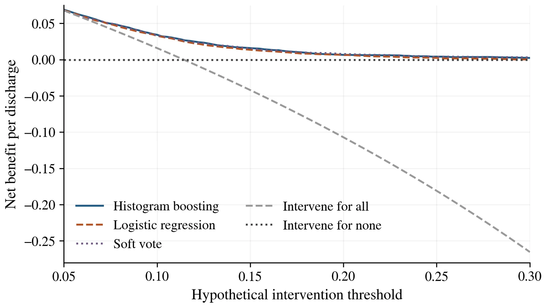
Decision curves were used to assess the hypothetical intervention thresholds between 0.05 and 0.30 based on net benefit as defined by Equation (6) [19]. TP(t) and FP(t) are the numbers of true and false positive alerts at threshold t. Under this interpretation, the assumed ratio of harm of a false positive is the multiplier t/(1−t). Each decision is attached to an encounter at discharge; therefore, it is possible that a patient can have more than one possible decision. No specific intervention, capacity constraint, clinical benefit, or monetary cost was measured.
NB(t) = TP(t) / N − FP(t) / N × t / (1 − t) (6)
The executed analysis used Python 3.12.14, scikit-learn 1.8.0, XGBoost 3.4.1, LightGBM 4.7.0, and SHAP 0.52.0. The notebook includes information about software versions, seeds of the random number generators, hashes of the input files, patient allocation, sampled search results, fitted thresholds, test probabilities, and output tables. All results reported here are from the standard configuration (three folds, three search candidates, 160 trees/iterations, and 500 bootstrap replicates) that was executed. There is no larger optional notebook configuration, nor is it represented as a completed experiment, for this paper.
4 Results
4.1 Cohort composition and data completeness
The number of age exclusions removed 852 encounters, and then the number of disposition exclusions removed 2,444 encounters, as shown in Table 1. At the end of the cohort, there were 11,260 recorded ERs for eligible encounters, which is 11.44% of all eligible encounters. The test partition comprised 19693 encounters from 13870 patients, 2252 events, and 17441 non-events. The prevalence was well distributed between the four partitions with values of ~11.43%, ~11.44%, ~11.43%, and ~11.44%, respectively. This similarity is not indicative of comparability with another hospital or later time period and reflects the stratified allocation. Data audit revealed missing weight in 96.86% of encounters, missing medical specialty in 49.08% of encounters, missing payer code in 39.56% of encounters, and missing race in 2.23% of encounters. These percentages are based on the supplied data set (original). The medical specialty was retained, even though it was missing, because the observed and missing categories may reflect referral and documentation patterns; the usefulness of this was tested within the administrative-family ablation. Keeping missing categories would not exclude entire cases but would not correct for any bias in documentation due to nonrandomness.
4.2 Model comparison and primary selection
The selection scores obtained in the training sets are now reported together with the results obtained with the independent test sets in Table 3. Before test evaluation, histogram gradient boosting has the best mean grouped cross-validation AP of 0.2227. The next best models were XGBoost with 0.2219 and random forest with 0.2205. Note that the relative size of the cross-validation means are small and thus should not be interpreted as definitive evidence of a universal algorithm ranking. The standard deviations are not confidence intervals but indicate variation across the three training folds.
Table 3. Training selection and independent test performance.
| Model | CV AP mean ± SD | Test AP 95% interval | Test AUROC | Test Brier |
|---|---|---|---|---|
| Logistic regression | 0.2119 ±0.0141 | 0.2078 (0.1877–0.2346) | 0.6598 | 0.0977 |
| Linear SVM | 0.2152 ±0.0130 | 0.2125 (0.1900–0.2407) | 0.6635 | 0.0976 |
| Gaussian naïve Bayes | 0.1944 ±0.0154 | 0.1916 (0.1716–0.2191) | 0.6426 | 0.0995 |
| Decision tree | 0.1968 ±0.0092 | 0.1987 (0.1786–0.2237) | 0.6507 | 0.0982 |
| Random forest | 0.2205 ±0.0170 | 0.2265 (0.2030–0.2557) | 0.6699 | 0.0967 |
| Extra trees | 0.2198 ±0.0125 | 0.2208 (0.1987–0.2507) | 0.6690 | 0.0972 |
| Histogram boosting* | 0.2227 ±0.0159 | 0.2258 (0.2034–0.2553) | 0.6704 | 0.0966 |
| XGBoost | 0.2219 ±0.0167 | 0.2226 (0.2020–0.2479) | 0.6693 | 0.0972 |
| LightGBM | 0.2186 ±0.0145 | 0.2172 (0.1948–0.2474) | 0.6651 | 0.0971 |
| Soft vote† | Not ranked | 0.2269 (0.2044–0.2549) | 0.6728 | 0.0969 |
| Prevalence baseline | Not ranked | 0.1144 (0.1083–0.1198) | 0.5000 | 0.1013 |
Primary model selected using training cross-validation. Secondary equal-weight ensemble of histogram boosting, XGBoost, and random forest. Intervals use 500 patient-cluster bootstrap replicates. All test probabilities in this table were calibrated independently. Higher AP and AUROC and lower Brier score are better; AP has a prevalence reference of 0.1144.
The selected model achieved test AP 0.2258 (95% interval 0.2034–0.2553), AUROC 0.6704 (0.6580–0.6842), and Brier score 0.0966 (0.0928–0.1001). Logistic regression achieved AP 0.2078, AUROC 0.6598, and Brier score 0.0977. Weaker but positive improvement in the prespecified comparison was supported by the paired AP difference of 0.0180 (95% interval 0.0118 to 0.0252) in this test sample. This allocation and limited tuning budget is a condition of this comparison. The largest test AP, 0.2269, and AUROC, 0.6728, were obtained from the secondary soft vote, and random forest had AP 0.2265. Advantages over the primary model of about 0.0011 and 0.0007 were achieved by their AP, respectively. These observations are clear but have not been used to re-label the chosen model. No pair of inferential claims about the vote or the forest that one is better than the other is offered. The prevalence baseline had an AP of 0.1144, an AUROC of 0.5000, and a Brier score of 0.1013.
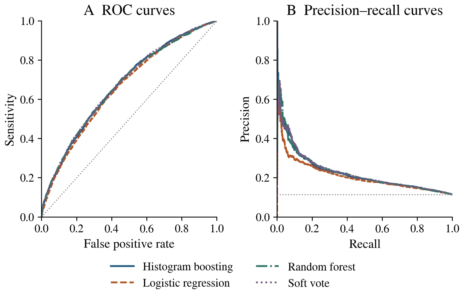
The chosen model and the secondary vote, along with the random forest model, are shown in Figure 2, while Table 3 shows all nine classifiers. The ROC curves are overlapping and indicate modest differences in discrimination. The precision–recall panel helps to make apparent the low precision at high recall. The horizontal dotted line represents the prevalence of the test event, and the ROC diagonal represents the chance ranking. Small numbers of observations at very high rank are represented by the irregular, high-precision, low-recall area and should not be considered as a stable operating region.
4.3 Threshold-dependent errors and calibration
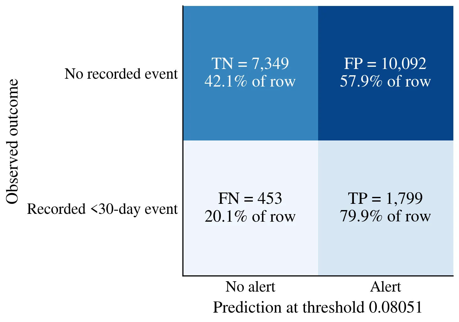
The threshold of the chosen model was 0.0805106. When applied to the test set, it achieved a sensitivity of 79.88%, a specificity of 42.14%, a precision of 15.13%, and an F1 score of 0.2544. Selected operating points under the common sensitivity-oriented selection rule are compared in Table 4. Sensitivities of the tests achieved are variable due to each threshold being set independently and each model's score distribution and generalization error varying. The selected model detected fewer events and produced fewer false positives compared to logistic regression.
Table 4. Test performance at independently chosen operating thresholds.
| Model | Sensitivity % | Specificity % | Precision % | F1 |
|---|---|---|---|---|
| Logistic regression | 80.95 | 38.68 | 14.56 | 0.2469 |
| Random forest | 79.93 | 41.98 | 15.10 | 0.2540 |
| Histogram boosting | 79.88 | 42.14 | 15.13 | 0.2544 |
| Soft vote | 79.53 | 42.50 | 15.15 | 0.2546 |
| Prevalence baseline | 100.00 | 0.00 | 11.44 | 0.2052 |
The threshold was chosen on the threshold partition to maximize specificity with a sensitivity ≥80% for each model. The constant prevalence model raises alarms on all test encounters in this policy, with zero specificity and high sensitivity.
The absolute counts are shown in Figure 3, as is the percentage of the counted values in each of the observed-outcome rows. A total of 1799 true positive alerts, 453 missed events, 10092 false positive alerts, and 7349 true negatives were identified. The rule detected 11,891 encounters (60.38% of the test set) and produced about 5.6 false positive alerts per encounter detected. The sensitivity-oriented policy has this workload as one of its main constraints. The overall accuracy of 46.45% is dependent on the threshold selected for interpretation and should be used in addition to the prespecified AP comparison.
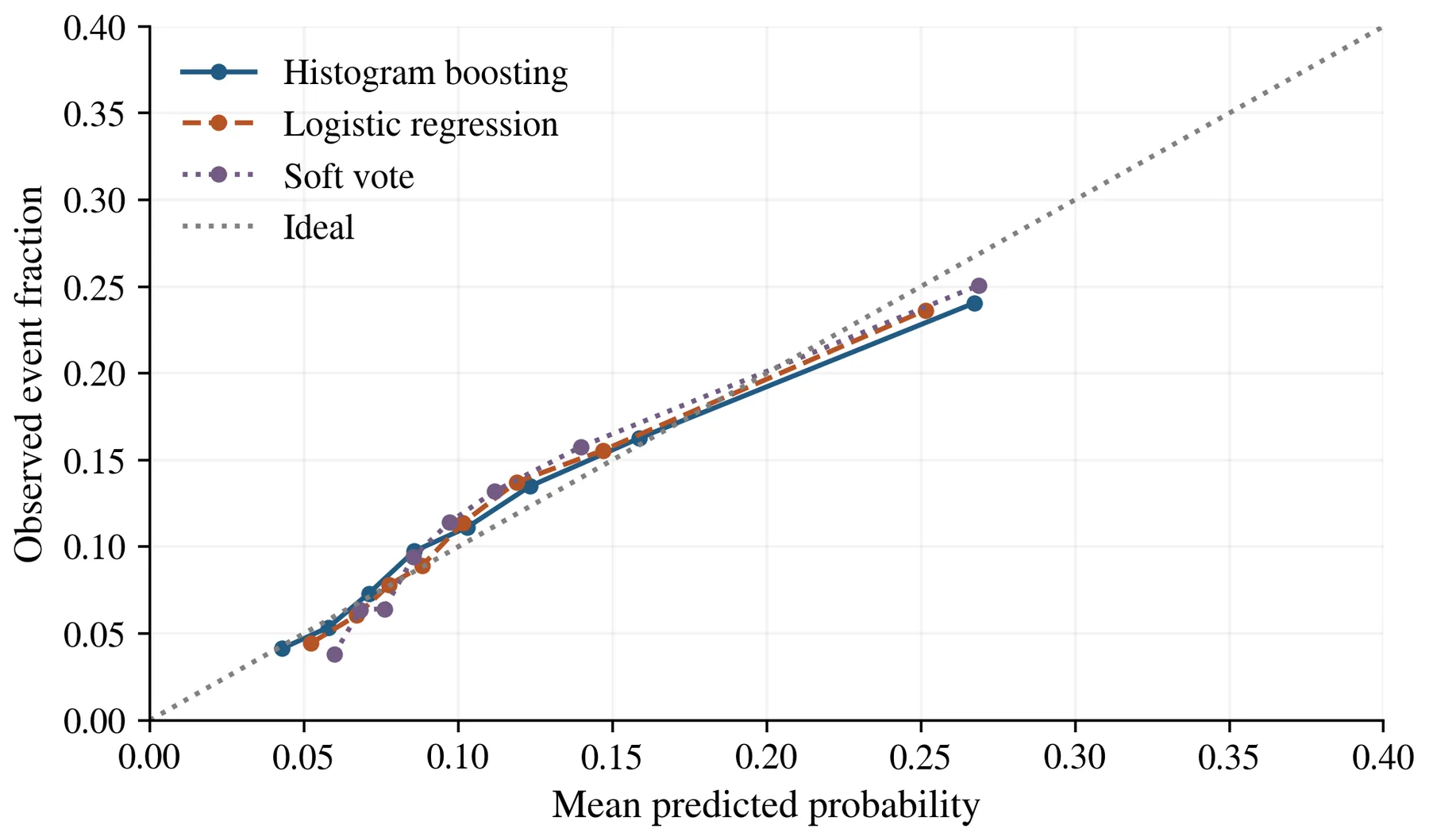
In Figure 4, eight quantile-bin averages of the selected model and logistic regression and the secondary vote are compared to the ideal diagonal. The minimum bin mean predicted risk was 4.30% with 4.14% observed frequency, and the maximum bin mean predicted risk was 26.73% with 24.05% observed frequency. The latter means overprediction for that combined risk stratum. There was residual calibration error with a test calibration intercept of −0.1246 and a test calibration slope of 0.9317. Bin averages cannot be connected to form a confidence band, nor to give reliability to each separate prediction. For no calibration ablation, AP and AUROC were kept the same since ranking was maintained by keeping the fitted sigmoid. The Brier score for it was 0.096604 and 0.096635 after calibration (a numerical difference that was very slight in favor of the uncalibrated probabilities), while log loss was 0.335567 and 0.335547 after calibration. So this run did not always improve the probability-error measures due to calibration. It takes this as a predefined procedure, and its empirical impact is reported without assuming that calibration needs to be improved with respect to every metric.
4.4 Ablation findings
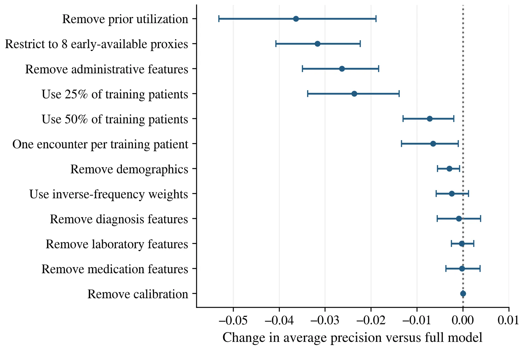
The entire chosen model and all 12 ablations are provided in Table 5. The highest level of AP reduction (from 0.2258 to 0.1894) came from the removal of prior utilization, and the removal of administrative features reduced AP to 0.1994. The proxy model with 8 limited features was able to get AP 0.1941. In these studies, the benefit of the full model is highly context-dependent with regard to encounter history and administration. They do not prove that each feature is a causal risk element or that the restricted model is ready for use at admission.
Table 5. Performance after predefined changes to the selected pipeline.
| Model variant | Test AP | Test AUROC | Test Brier |
|---|---|---|---|
| Full model | 0.2258 | 0.6704 | 0.0966 |
| Remove prior utilization. | 0.1894 | 0.6294 | 0.0987 |
| Remove diagnosis. | 0.2249 | 0.6673 | 0.0967 |
| Remove medication | 0.2255 | 0.6680 | 0.0967 |
| Remove laboratory | 0.2255 | 0.6719 | 0.0966 |
| Remove demographics. | 0.2228 | 0.6688 | 0.0968 |
| Remove administrative | 0.1994 | 0.6439 | 0.0981 |
| Restrict to 8 early-available proxies. | 0.1941 | 0.6242 | 0.0985 |
| Inverse-frequency weights | 0.2234 | 0.6705 | 0.0967 |
| 25% of training patients | 0.2021 | 0.6587 | 0.0978 |
| 50% of training patients | 0.2185 | 0.6674 | 0.0969 |
| One random encounter per training patient | 0.2193 | 0.6671 | 0.0969 |
| Remove calibration. | 0.2258 | 0.6704 | 0.0966 |
The same test patients are used for all variants. The fixed hyperparameters of the selected classifier were used to retrain it, except for removing the calibration. Reduced training sets were sampled per patient, and for each variant it was calibrated (and a threshold fitted if applicable). Removal of families does not mean independent causal action.
Figure 5 shows each paired difference of the ablations from the full model on a common scale. Horizontal intervals are 95% patient-cluster bootstrap intervals, and the vertical line at zero indicates no observed AP difference. Removing prior utilization changed AP by −0.0364 (interval −0.0532 to −0.0189), and removing administrative features by −0.0264 (−0.0350 to −0.0183). By contrast, intervals for getting rid of medicine, lab, and diagnosis features contained no zeroes. These comparisons are descriptive and not adjusted; the number should not be interpreted as 12 individual hypothesis tests. The AP for 25% and 50% patients were 0.2021 and 0.2185, respectively, while for all the patients it was 0.2258. Randomly selected one training encounter per patient yielded AP 0.2193. This fitted model was determined by the differences, which indicates that both sample size and retained encounter information influenced this fitted model, but with one seeded subsample and not repeated learning-curve experiments. The inverse-frequency training weights yielded the AP score of 0.2234, which was not better than the unweighted model. The relatively minimal adjustments made following the deletion of a few clinical feature families are not indicative of clinical irrelevance but may reflect redundancy or coarse measurement.
4.5 Explanations and performance heterogeneity
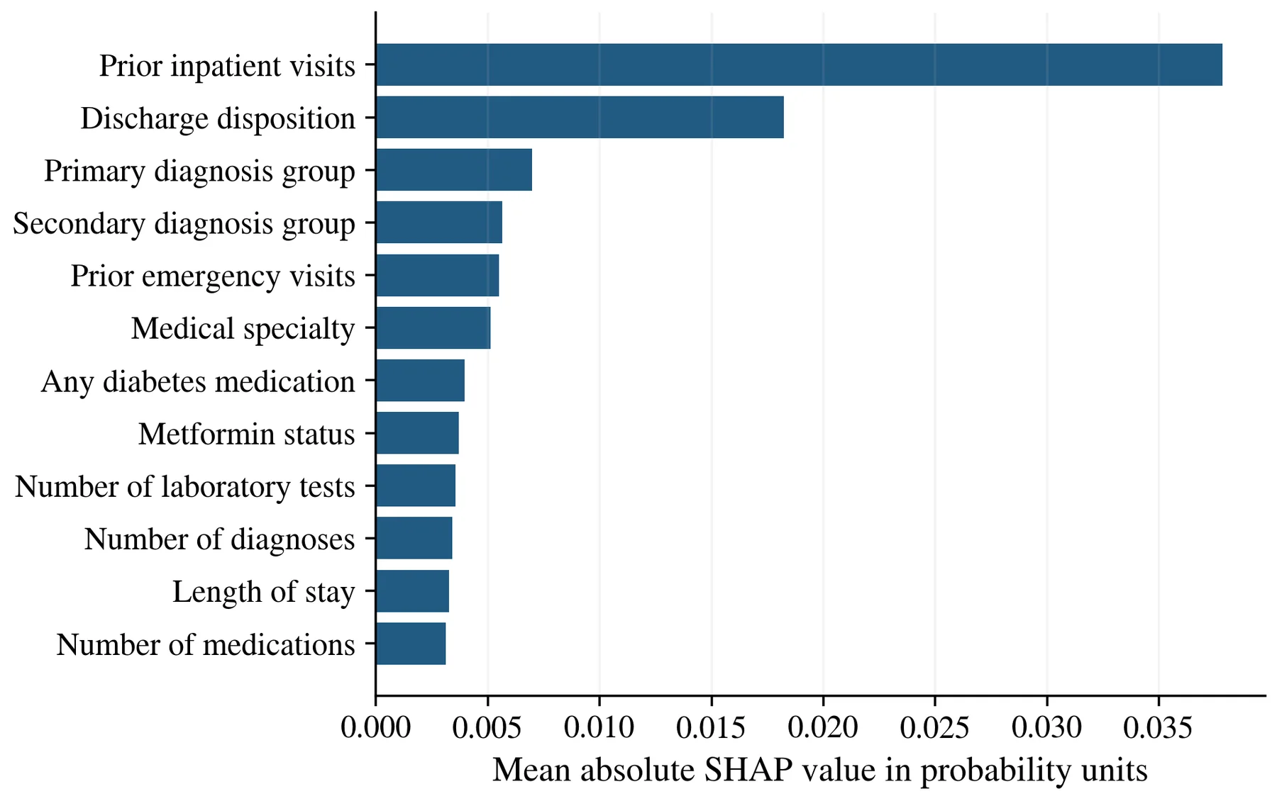
The 12 most significant feature attributions (in the mean absolute sense) provided by the calibrated selected model are shown in Figure 6. The most influential visits were previous inpatient visits with a probability unit of 0.03785 and discharge disposition with a probability unit of 0.01824. Medical specialty was followed by prior emergency visits (0.00563) and primary and secondary diagnosis groups (0.00698 and 0.00550, respectively). A larger bar does not represent that a feature consistently increases risk—it simply reflects a higher magnitude of contribution compared to the sampled background. The sequences reasonably reflect the uses and administrative amputations. SHAP and ablation results are different answers to different questions. A diagnosis can affect individual predictions even when other variables make up for it and the entire diagnosis family is omitted from the model and retrained. On the other hand, there is no guarantee that altering a feature with a high importance would alter the patient's outcome. Numerical verification of local additivity was made; the maximum value of the residual is approximately 3.3 × 10⁻¹⁶, but this does not guarantee the stability of the attribution or the clinical validity. Only 80 encounters have been randomly sampled and ranked worldwide.
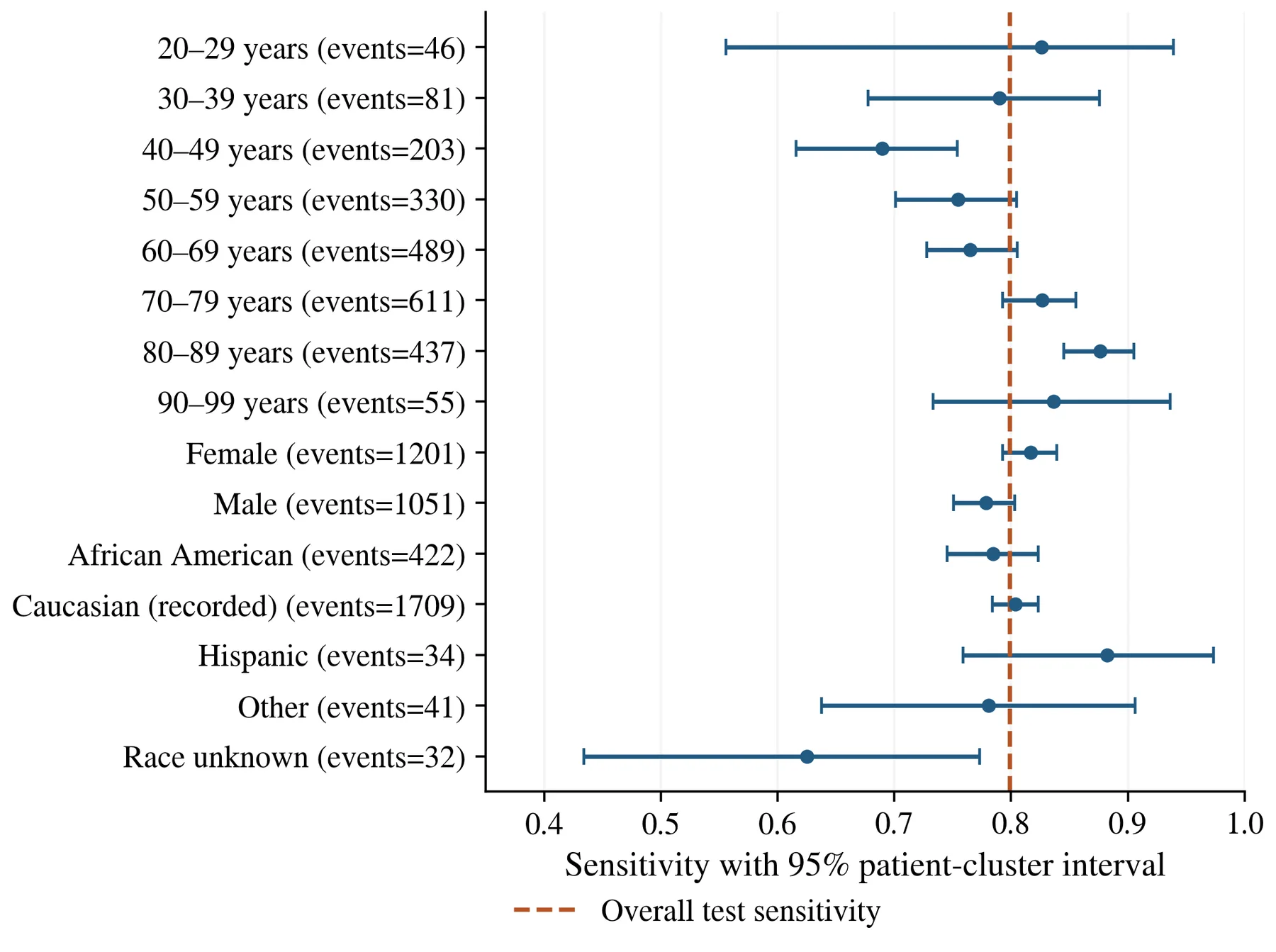
Subgroup sensitivity is displayed in Figure 7 in terms of patient-cluster intervals and event counts. Records with a female label achieved a sensitivity of 81.68%, and records with a male label achieved a sensitivity of 77.83%. Across age bands it ranged from 68.97% at ages 40–49 to 87.64% at ages 80–89. The recorded groups of African Americans and Caucasians had sensitivity values of 78.44% and 80.34%, respectively. Smaller group intervals are shown with wide intervals to demonstrate why apparent differences should be interpreted with caution. Only 14 events were in the Asian subgroup, and its performance measures were suppressed by the predefined rule. Categories are a reproduction of the original coding and are not to be interpreted as biological explanations of risk.
The home-related discharge subset included 14,315 test encounters and 1,415 events with an AP of 0.1991 and sensitivity of 70.04%. Other qualified discharges were 96.54% sensitive but just 7.86% specific. This strong threshold behavior is consistent with discharge disposition being a strong model input and implies that the overall sensitivity target does not apply to all care settings in the same way. Equal-patient weighting of the selected model resulted in 0.1704 AP, 0.6877 AUROC, and 0.0669 Brier score. This change in case mix is one factor that helps explain why these two AP values should not be compared as if they represented the same target population, as the corresponding weighted event prevalence was 0.0748, compared with 0.1144 under equal-encounter weighting.
4.6 Exploratory decision curves
Risk-based alerting and hypothetical intervention (all or none) are shown in Figure 8. For the selected model, net benefit was 0.0344 per discharge at threshold 0.10, 0.0160 at 0.15, and 0.0067 at 0.20. The selected model and the vote generally had similar curves, and the numerical gap to logistic regression was small. These values represent the assumed tradeoff in Equation (6) and not an actual reduction in readmissions. No uncertainty bands, future intervention outcomes, or implementation costs were estimated, and a positive net benefit using this calculation is not enough to determine clinical effectiveness.
5 Discussion
5.1 Main findings and comparison with earlier work
The main impact is that the histogram gradient boosting model shows a slight increase of AP over logistic regression for the patient-separated internal evaluation. The AUROC of 0.6704 suggests it has limited to moderate discrimination and not high individual forecasting power. The secondary vote and random forest slightly outperformed in terms of the observed test AP, thus corroborating the finding that multiple tree-based methods were comparable in the limited search space. The value of the analysis is that these differences are quantifiable in addition to the value of the calibration, errors, and dependence on the information families used. Selected earlier results are provided in Table 6, which do not represent a pooled benchmark. Internal and external discrimination of the DERRI studies were different and significant [2], [7]. The present result is not conclusive for superiority over such models due to the different sets of predictors, event capture, prevalence, and validation population. Instead, the comparison is meant to show why one result from one historical source should not be assumed to apply to another setting.
Table 6. Contextual comparison with selected previous studies.
| Study | Data and evaluation | Reported finding |
|---|---|---|
| DERRI development [2] | 44,203 discharges; clinical development and validation samples | Validation C statistic 0.69 |
| DERRI external evaluation [7] | 105,974 discharges; external cohort | C statistic 0.634 |
| UCI comparison in 2021 [8] | 100,244 retained records; three classifier families | Random forest ranked highest by AUC |
| UCI comparison in 2024 [9] | UCI data; feature optimization, grouped cross-validation, and SMOTE | Tree ensembles were competitive |
| UCI framework in 2026 [11] | UCI data; nested cross-validation and calibrated analysis | Stacking AUROC 0.664 and 0.688 in the respective analyses |
| Present study | 98,470 eligible encounters; four patient-separated partitions | Selected model test AUROC 0.6704; AP 0.2258. |
Random forests and methods based on boosting have been previously noted to perform well in UCI benchmarks [8] and [9]. Our results agree with the general statement but only indicate slight variations between the top ensembles. The genetic-algorithm study focused on maximizing threshold-dependent classification metrics [10], and the selection of models in this study was based on AP and a threshold determined independently, based on the natural test prevalence. F1 scores, or accuracy, of different resampling and threshold policies cannot be directly compared to the values in Table 4. Nested cross-validation, calibration, decision analysis, and SHAP were already a part of the 2026 framework [11]. The unique methodological aspects of our study are thus the four-part patient allocation and the paired feature-family and training-data ablations. Also, the single locked holdout is different than repeatedly outer-fold evaluation. Not a methodological or empirical leap that this paper is introducing explainable readmission modeling, or that it is providing the best possible ensemble architecture.
5.2 Interpretation of feature contributions
The highest SHAP value and removal-associated AP loss was observed for prior utilization. This agreement indicates that earlier inpatient and emergency contact summarizes information relevant to the recorded outcome that isn't fully captured by the diagnosis and medication categories available. The administrative ablation was also significant, and the large difference between home and other discharges indicates that discharge context influences both threshold behavior and ranking. These variables can relate to burden of illness, organization of services, documentation, or access to follow-up, and the current data does not distinguish these effects. This is not in conflict with the source study investigating HbA1C measurement and readmission [4] because the small AP change after laboratory feature removal did not alter the results of the study.
The association between a particular measurement process and a measurement is not the same as the incremental prediction of the measurement process given multiple correlated inputs. Likewise, little indication of medication-family ablation effects does not mean that medication management is not important to patients. The variables reported are very broad, and this observational comparison does not provide an estimate of the treatment benefit or change in care consequences. The no-calibration result is informative, too. Independent calibration is a safe development step, but whether or not it is useful is an empirical question and cannot be taken for granted [17], [27]. Here, there was no change in the ranking, and the two probability-error measures shifted slightly in opposite directions.
Even with the highest risk bin shown, there is some degree of overprediction, which indicates that risk predictions would still need to be evaluated and updated in a modern population for deployment.
5.3 Practical meaning of the operating policy
With a sensitivity of approximately 80%, over three-fifths of test encounters resulted in an alert, and only about one in seven resulted in a recorded early readmission. This operating point may present a a potential workload if it takes a lot of staff time and an intervention is needed. A different capacity or a harm tradeoff for the same model could support a different use, but the current analysis does not provide a policy for this. The choice of threshold should be associated with an intervention and judged in the future direction; the threshold alone, without the intervention, does not show clinical value. A single operating point in the aggregate is also not easy to interpret because of the effects of subgroup variation. There was a significant variation in the sensitivity of the same threshold for different discharge settings and age bands. Some of the race categories have small numbers of records, and there are some repeated records; this means the precision cannot be guaranteed or that an unchanging demographic label cannot be assumed for all patients. Recorded categories, missingness, and access-related outcome capture require separate investigation. Not giving any features related to race the same weight would not be fair, as correlated features and the outcome itself can carry unequal healthcare experiences [32].
5.4 Limitations and future work
First, this is a historical secondary analysis based on records from the years 1999-2008. Coding and treatment patterns, discharge arrangements, and data capture have changed, and no modern external validation took place. Identifiers and dates are not included in the public files, which restricts the ability to hospital hold out and/or temporally evaluate. Patient-separated validation deals with one of the key dependence structures but does not resolve site-level and time-related dependence structures.
Secondly, it results in a recorded readmission category, and incomplete knowledge of care outside the contributing source. The planning of admissions, post-discharge fatalities, and incomplete follow-up cannot be properly addressed. There is an age restriction (not including patients aged 18–19) and source inclusion criteria that exclude other inpatient populations. Care pathways or documentation practices that don't transport reliably may be coded in retained transfer dispositions and missing medical specialties. The limitations refer to the target to be predicted and cannot be overcome simply by elaborate modeling. Third, only three hyperparameter settings for each model and three folds of training were tested. This ranking is based on a small search and only one partition seed and is not a comprehensive evaluation of the potential of an algorithm.
The independent calibration and threshold partitions increase the separation of the decisions and decrease the number of observations for base-model fitting. Only 500 replicates are used to make bootstrap intervals, so they represent the variation among test patients given the fixed models. They do not account for training variability, hospital clustering, or multiplicity adjustment for exploratory comparisons. Fourth, ablations keep fixed the hyperparameters that they select and sample the training data using the same single seed and thus cannot be interpreted as optimized reduced models or entire learning curves. SHAP estimates rely on a small background and explanation sample, independence-based masking, and small permutations. These limitations are not overcome by having good numerical additivity.
Subgroup analyses provide a descriptive performance, and utility was assessed without quantification of an intervention, and intersectional performance was not estimated. Future studies should first secure records that have an explicitly defined intervention opportunity with reliable hospital membership, complete follow-up, and event timing. Then, it should consider both temporal and external transportability, group development of models across seeds or outer folds, extend budgets of tuning and resampling, and examine explanation stability. A separate study of admission time is required, with the restricted feature analysis only informing the other study, once it is determined when the various inputs are available. Volume of alerts, consequences of subgroups, resource utilization, and patient outcomes should be measured in prospective assessment prior to deployment claim.
6 Conclusion
Histogram gradient boosting outperformed logistic regression with a marginal test boost in AP on 98,470 eligible encounters from the UCI Diabetes 130-US Hospitals dataset, while having the best training cross-validation AP. It had an AP of 0.2258 and an AUROC of 0.6704 with a significant false-positive burden at a threshold adjusted to 80% sensitivity. The fitted model was more clearly associated with prior use and administrative information than with the incremental information provided by a number of diabetes-specific families of features. The study is a reproducible comparative analysis of readmission after discharge and does not determine prediction of diabetes onset, transportability to existing hospitals, or clinical effectiveness.
Data availability
It is publicly available from the UCI Machine Learning Repository as the source dataset and administrative mapping file for the dataset record “Diabetes 130-US Hospitals for Years 1999-2008”, DOI 10.24432/C5230J [3].
Ethical considerations and declarations
This study was based on publicly available, de-identified secondary data and did not require the recruitment, contact with, or intervention with participants. Only to counteract the effect of repeated encounters and to resolve the potential overlap of partitions, the following patient identifiers were used as their source. No attempt was made at reidentification. An institutional ethics approval or exemption is not provided and not claimed. Author affiliations, funding, competing interests, and any necessary institutional determination have to be established by the authors prior to submission.
References
- [1] Kansagara D, Englander H, Salanitro A, Kagen D, Theobald C, Freeman M, Kripalani S. Risk prediction models for hospital readmission: a systematic review. JAMA. 2011;306(15):1688–1698. https://doi.org/10.1001/jama.2011.1515
- [2] Rubin DJ, Handorf EA, Golden SH, Nelson DB, McDonnell ME, Zhao H. Development and Validation of a Novel Tool to Predict Hospital Readmission Risk Among Patients with Diabetes. Endocrine Practice. 2016;22(10):1204-1215. https://doi.org/10.4158/e161391.or
- [3] Clore J, Cios K, DeShazo J, Strack B. Diabetes 130-US Hospitals for Years 1999-2008. UCI Machine Learning Repository. 2014. https://doi.org/10.24432/C5230J
- [4] Strack B, DeShazo JP, Gennings C, Olmo JL, Ventura S, Cios KJ, Clore JN. Impact of HbA1c Measurement on Hospital Readmission Rates: Analysis of 70,000 Clinical Database Patient Records. BioMed Research International. 2014;2014:781670. https://doi.org/10.1155/2014/781670
- [5] Futoma J, Morris J, Lucas J. A comparison of models for predicting early hospital readmissions. Journal of Biomedical Informatics. 2015;56:229-238. https://doi.org/10.1016/j.jbi.2015.05.016
- [6] Christodoulou E, Ma J, Collins GS, Steyerberg EW, Verbakel JY, Van Calster B. A systematic review shows no performance benefit of machine learning over logistic regression for clinical prediction models. Journal of Clinical Epidemiology. 2019;110:12-22. https://doi.org/10.1016/j.jclinepi.2019.02.004
- [7] Rubin DJ, Recco D, Turchin A, Zhao H, Golden SH. External Validation of the Diabetes Early Re-Admission Risk Indicator (Derri™). Endocrine Practice. 2018;24(6):527-541. https://doi.org/10.4158/ep-2018-0035
- [8] Shang Y, Jiang K, Wang L, Zhang Z, Zhou S, Liu Y, Dong J, Wu H. The 30-days hospital readmission risk in diabetic patients: predictive modeling with machine learning classifiers. BMC Medical Informatics and Decision Making. 2021;21(S2):57. https://doi.org/10.1186/s12911-021-01423-y
- [9] Liu VB, Sue LY, Wu Y. Comparison of machine learning models for predicting 30-day readmission rates for patients with diabetes. Journal of Medical Artificial Intelligence. 2024;7:23. https://doi.org/10.21037/jmai-24-70
- [10] Zeinalnezhad M, Shishehchi S. An integrated data mining algorithms and meta-heuristic technique to predict the readmission risk of diabetic patients. Healthcare Analytics. 2024;5:100292. https://doi.org/10.1016/j.health.2023.100292
- [11] Salim SS, Ibrahim AA. A Machine Learning Approach for Predicting 30-Day Hospital Readmission in Patients with Diabetes. Healthcare. 2026;14(9):1185. https://doi.org/10.3390/healthcare14091185
- [12] Varma S, Simon R. Bias in error estimation when using cross-validation for model selection. BMC Bioinformatics. 2006;7(1):91. https://doi.org/10.1186/1471-2105-7-91
- [13] Roberts DR, Bahn V, Ciuti S, Boyce MS, Elith J, Guillera‐Arroita G, Hauenstein S, Lahoz‐Monfort JJ, Schröder B, Thuiller W, Warton DI, Wintle BA, Hartig F, Dormann CF. Cross‐validation strategies for data with temporal, spatial, hierarchical, or phylogenetic structure. Ecography. 2017;40(8):913-929. https://doi.org/10.1111/ecog.02881
- [14] Kapoor S, Narayanan A. Leakage and the reproducibility crisis in machine-learning-based science. Patterns. 2023;4(9):100804. https://doi.org/10.1016/j.patter.2023.100804
- [15] Saito T, Rehmsmeier M. The Precision-Recall Plot Is More Informative than the ROC Plot When Evaluating Binary Classifiers on Imbalanced Datasets. PLOS ONE. 2015;10(3):e0118432. https://doi.org/10.1371/journal.pone.0118432
- [16] Davis J, Goadrich M. The relationship between Precision-Recall and ROC curves. Proceedings of the 23rd international conference on Machine learning - ICML '06. 2006:233-240. https://doi.org/10.1145/1143844.1143874
- [17] Van Calster B, McLernon DJ, van Smeden M, Wynants L, Steyerberg EW, On behalf of Topic Group ‘Evaluating diagnostic tests and prediction models’ of the STRATOS initiative. Calibration: the Achilles heel of predictive analytics. BMC Medicine. 2019;17(1):230. https://doi.org/10.1186/s12916-019-1466-7
- [18] Steyerberg EW, Vickers AJ, Cook NR, Gerds T, Gonen M, Obuchowski N, Pencina MJ, Kattan MW. Assessing the performance of prediction models: a framework for traditional and novel measures. Epidemiology. 2010;21(1):128-138. https://doi.org/10.1097/ede.0b013e3181c30fb2
- [19] Vickers AJ, Elkin EB. Decision Curve Analysis: A Novel Method for Evaluating Prediction Models. Medical Decision Making. 2006;26(6):565-574. https://doi.org/10.1177/0272989x06295361
- [20] Collins GS, Moons KGM, Dhiman P, Riley RD, Beam AL, Van Calster B, Ghassemi M, Liu X, Reitsma JB, van Smeden M, Boulesteix AL, Camaradou JC, Celi LA, Denaxas S, Denniston AK, Glocker B, Golub RM, Harvey H, Heinze G, Hoffman MM, Kengne AP, Lam E, Lee N, Loder EW, Maier-Hein L, Mateen BA, McCradden MD, Oakden-Rayner L, Ordish J, Parnell R, Rose S, Singh K, Wynants L, Logullo P. TRIPOD+AI statement: updated guidance for reporting clinical prediction models that use regression or machine learning methods. BMJ. 2024;385:e078378. https://doi.org/10.1136/bmj-2023-078378
- [21] Moons KGM, Damen JAA, Kaul T, Hooft L, Andaur Navarro C, Dhiman P, Beam AL, Van Calster B, Celi LA, Denaxas S, Denniston AK, Ghassemi M, Heinze G, Kengne AP, Maier-Hein L, Liu X, Logullo P, McCradden MD, Liu N, Oakden-Rayner L, Singh K, Ting DS, Wynants L, Yang B, Reitsma JB, Riley RD, Collins GS, van Smeden M. PROBAST+AI: an updated quality, risk of bias, and applicability assessment tool for prediction models using regression or artificial intelligence methods. BMJ. 2025;388:e082505. https://doi.org/10.1136/bmj-2024-082505
- [22] Cortes C, Vapnik V. Support-vector networks. Machine Learning. 1995;20(3):273-297. https://doi.org/10.1007/bf00994018
- [23] Breiman L. Random Forests. Machine Learning. 2001;45(1):5-32. https://doi.org/10.1023/a:1010933404324
- [24] Geurts P, Ernst D, Wehenkel L. Extremely randomized trees. Machine Learning. 2006;63(1):3-42. https://doi.org/10.1007/s10994-006-6226-1
- [25] Friedman JH. Greedy function approximation: A gradient boosting machine. The Annals of Statistics. 2001;29(5):1189–1232. https://doi.org/10.1214/aos/1013203451
- [26] Chen T, Guestrin C. XGBoost: A scalable tree boosting system. Proceedings of the 22nd ACM SIGKDD International Conference on Knowledge Discovery and Data Mining. 2016:785-794. https://doi.org/10.1145/2939672.2939785
- [27] Niculescu-Mizil A, Caruana R. Predicting good probabilities with supervised learning. Proceedings of the 22nd international conference on Machine learning - ICML '05. 2005:625-632. https://doi.org/10.1145/1102351.1102430
- [28] Efron B. Bootstrap Methods: Another Look at the Jackknife. The Annals of Statistics. 1979;7(1):1–26. https://doi.org/10.1214/aos/1176344552
- [29] Riley RD, Ensor J, Snell KIE, Harrell FE, Martin GP, Reitsma JB, Moons KGM, Collins G, van Smeden M. Calculating the sample size required for developing a clinical prediction model. BMJ. 2020;368:m441. https://doi.org/10.1136/bmj.m441
- [30] Lundberg SM, Erion G, Chen H, DeGrave A, Prutkin JM, Nair B, Katz R, Himmelfarb J, Bansal N, Lee SI. From local explanations to global understanding with explainable AI for trees. Nature Machine Intelligence. 2020;2(1):56-67. https://doi.org/10.1038/s42256-019-0138-9
- [31] Aas K, Jullum M, Løland A. Explaining individual predictions when features are dependent: More accurate approximations to Shapley values. Artificial Intelligence. 2021;298:103502. https://doi.org/10.1016/j.artint.2021.103502
- [32] Obermeyer Z, Powers B, Vogeli C, Mullainathan S. Dissecting racial bias in an algorithm used to manage the health of populations. Science. 2019;366(6464):447-453. https://doi.org/10.1126/science.aax2342
CITE THIS ARTICLE
Dey, T. (2026). A Comparative Study of Machine Learning Algorithms for Early Disease Prediction Using Public Healthcare Datasets. https://www.researchbytresna.com/article/07c95d48-df6f-454f-8a04-d8d9840bf92e
T. Dey, “A Comparative Study of Machine Learning Algorithms for Early Disease Prediction Using Public Healthcare Datasets,” 2026. [Online]. Available: https://www.researchbytresna.com/article/07c95d48-df6f-454f-8a04-d8d9840bf92e
Dey, T. (2026) ‘A Comparative Study of Machine Learning Algorithms for Early Disease Prediction Using Public Healthcare Datasets’. Available at: https://www.researchbytresna.com/article/07c95d48-df6f-454f-8a04-d8d9840bf92e
Dey, Tresna. “A Comparative Study of Machine Learning Algorithms for Early Disease Prediction Using Public Healthcare Datasets.” 2026, https://www.researchbytresna.com/article/07c95d48-df6f-454f-8a04-d8d9840bf92e.
Tresna Dey. “A Comparative Study of Machine Learning Algorithms for Early Disease Prediction Using Public Healthcare Datasets.” (2026). https://www.researchbytresna.com/article/07c95d48-df6f-454f-8a04-d8d9840bf92e.
Dey T. A Comparative Study of Machine Learning Algorithms for Early Disease Prediction Using Public Healthcare Datasets. 2026. https://www.researchbytresna.com/article/07c95d48-df6f-454f-8a04-d8d9840bf92e
@misc{article_07c95d48df6f454f8a04d8d9840bf92e,
  title = {A Comparative Study of Machine Learning Algorithms for Early Disease Prediction Using Public Healthcare Datasets},
  author = {Tresna Dey},
  year = {2026},
  url = {https://www.researchbytresna.com/article/07c95d48-df6f-454f-8a04-d8d9840bf92e},
}
TY - GEN AU - Tresna Dey TI - A Comparative Study of Machine Learning Algorithms for Early Disease Prediction Using Public Healthcare Datasets PY - 2026 UR - https://www.researchbytresna.com/article/07c95d48-df6f-454f-8a04-d8d9840bf92e ER -