The challenge of comparative prediction studies for diabetes must be evaluated in terms of discrimination and whether any improvement over the algorithm is maintained over time or is converted to meaningful probabilities. In this study, six supervised learning models were compared and evaluated, involving the same participants and predictors, and inference was performed using a survey in addition to a later-period test set. Methods: NHANES 2007–2018 provided 31,772 adults aged at least 20 years. Development used 2007–2014 (n = 21,532), with separate fitting and calibration partitions; temporal testing used 2015–2018 (n = 10,240). Logistic regression, support vector machine, random forest, XGBoost, CatBoost, and multilayer perceptron were compared using 11 non-laboratory predictors and 13 predictors that included two lipid measurements. The outcome combined diagnosed diabetes, diabetes medication use, and HbA1c ≥6.5%; glycemic and diagnostic variables were excluded from predictors. Weighted discrimination, calibration, 1000 bootstrap replications from the survey, subgroup analysis, SHAP, and ablations were all included in the evaluation. Results: Laboratory-augmented CatBoost achieved ROC-AUC 0.836 (95% CI 0.821–0.852), average precision 0.465, and Brier score 0.0994. Its AUC exceeded logistic regression by 0.0139 (95% CI 0.0081–0.0197; Holm-adjusted p = 0.00012). AUC values were 0.809 for CatBoost (no significant difference with logistic regression after adjustment [p = 0.138]). The addition of lipids improved the CatBoost AUC by 0.0271. The calibration slope was 0.877, and the sensitivity at the common threshold was 38.6% for adults aged 20-44 years and 89.0% for those aged at least 65 years. Conclusions: Nonlinear models gained little from lipid information, and non-laboratory performance was similar to logistic regression. Screening interpretation is limited by limitations in calibration and sensitivity that vary by age. These results are for diabetes prevalence, not incident diabetes.
Research ArticleClinical Machine LearningIn progress
Performance Analysis of Supervised Learning Models for Diabetes Risk Prediction
Correspondence: tresnadey98@gmail.com
Abstract
Keywords diabetes risk predictionNHANESsupervised learningtemporal validationcalibrationsurvey weightingexplainable machine learning
1. Introduction
Diabetes places significant burdens on requiring chronic treatment and causing vascular and metabolic complications. International estimates suggest that the prevalence of this problem is large and increasing [1] and repeated surveys in the United States have shown that the prevalence of diabetes and control of risk factors remains problematic [2]. There are accessible assessment methods that could be used to identify individuals who should go for confirmatory testing. A statistical prediction, however, does not equal a clinical diagnosis. Diagnostic criteria and the contexts in which they need to be confirmed must not be confused with the "outcome" of an algorithm [3]. Supervised learning can be used to integrate demographic, anthropometric, behavioral, and clinical data to make predictions about diabetes-related outcomes.
It is attractive because it allows for the modelling of nonlinear relationships and interactions without needing all functional forms to be known in advance. However, an improvement on one accuracy estimate is not sufficient to create a useful model. A common outcome, predictor information, and the same validation population (which is independent of the development decisions) plus tuning are required for a fair comparison. Transparent reporting of these choices is at the heart of the ongoing TRIPOD+AI guidance [4]. Another systematic evidence indicates that machine learning is not necessarily superior to logistic regression when methodological biases are avoided in comparisons [5]. Discrimination and calibration are two different questions. A model can rank individuals fairly well but systematically overestimate or underestimate absolute probabilities.
This distinction is important when converting probabilities to screening thresholds, as an apparently good AUC may go hand in hand with an inappropriate operating point [6]. It also is relevant under temporal change: later survey participants might have a different prevalence of disease and/or exposure to treatment and measured risk factors, even if data is collected within the same national survey program. NHANES provides a suitable platform where, upon a controlled comparison, it is possible, as it incorporates questionnaires, examinations, and laboratory information. There are already works in which support vector machines and ensemble methods are used for diabetes classification [7], [8] and a recent one in which the same period (2007-2018) is used to compare models for diabetes classification based on lifestyles [9].
Newer diabetes-related models have also included external validation and calibration assessment [10]. The current research's contribution is a unique, reproducible set of survey-weighted temporal testing, matched feature scenarios, multiplicity-adjusted comparisons, and probability diagnostics and group operating characteristics. It is not based on a new algorithm or the idea that temporal validation has not been applied before. In this paper, “diabetes risk prediction” refers to the risk of diabetes at the assessment time. Observations are NOT longitudinal follow-ups of previously disease-free individuals but rather repeated cross-sectional samples. Analysis thus compares the diagnostic classification for subsequent survey cycles and does not provide an estimate of future incidence of diabetes.
1.1 Objective and research questions
The goal was to assess if supervised learning models offer improvements over logistic regression in the classification of prevalent diabetes, which are reproducible across predictor scenarios, probability calibration, and clinically relevant subgroups.
RQ1. Which model has the largest discrimination and correctly predicted probability in the later NHANES test population?
RQ2. Are nonlinear models superior to logistic regression post survey-aware paired inference and multiplicity adjustment?
RQ3. What is the contribution of lipid measures to prediction without laboratory measures, and what are the groups of features that explain the performance?
RQ4. Are the calibration and performance (depending on the threshold) stable between survey cycles by sex, age groups, and BMI groups?
2 Literature Review
2.1 Established diabetes risk assessment
Different tasks in diabetes prediction research include incident disease prediction, detection of undiagnosed diabetes, and identification of combined prediabetes/diabetes. Major heterogeneity in population, prediction variables, and validation techniques was identified in a systematic review of risk models [11]. This heterogeneity matters because models that target different outcomes cannot be ranked together in terms of performance. The Finnish Diabetes Risk Score is a prospective risk-assessment approach [12], and a United States self-assessment score was developed based on NHANES 1999-2004 and tested in NHANES 2005-2010 and independent community populations [13]. The latter study found that at its chosen score cut-off, the sensitivity was 79% and the specificity was 67% for NHANES. The target was free of known diabetes, which is not the case for the prevalent-diabetes phenotype studied here.
These studies show that low-burden predictors and validation beyond the development sample are nothing new. What remains relevant to them today is the connection between the purpose of the screening task, access to the predictor, and an explicit criterion for operating. An algorithmic comparison in modern times shouldn't break that connection but should not make a high AUC a sufficient endpoint.
2.2 Machine learning studies using population data
An early NHANES analysis was applied using support vector machines with both demographic and anthropometric and health-history predictors and achieved an AUC value of 0.835 for diabetes versus non-diabetes and 0.732 for classification into the combined undiagnosed diabetes/prediabetes category [7]. A subsequent NHANES-based data-driven study has performed a comparison between regression, support vector machines, and tree-based methods on wide sets of features. In that study under classification and validation design, the AUC of XGBoost was 0.862 without laboratory variables and 0.957 with laboratory information for the classification of diabetes [8]. It uses a balanced splitting strategy and feature search, rather than a compact feature set and population evaluation in the later cycle as is done here.
Researchers used NHANES 2007–2018 data to investigate and compare five algorithms that rely on lifestyle and related non-invasive information for 29,509 adults in 2025. Although XGBoost had an AUC of 0.8168, many of the combinations of the models and thresholds had low sensitivity and high specificity [9]. This contrast provides an impetus to report operating characteristics as well as discrimination. Finally, the present analysis evaluates objective HbA1c-based case identification, explicit survey-weighted paired comparisons, and the incremental information from two lipid measures, which also precludes a numerical claim of superiority over that study. Recent research has gone beyond the art of internal comparison. This 7-parameter model for prevalent prediabetes or diabetes was externally validated in NHANES 2021-2023 (AUC 0.773) and Korea NHANES (AUC 0.780) [10].
Another study externally validated an approximation model for prediabetes based on an EHR in the NHANES and explored discrimination, calibration, and recalibration [14]. As illustrated in these examples, validation and calibration are well established elements of the literature and are independent. This study instead queries whether or not the relative effectiveness of six algorithms is affected by the use and/or exclusion of lipid information for the same adult population.
2.3 Evaluation gaps and the contribution of this study
It is important to differentiate between ranking, accuracy of the probability, and the implications of making a threshold decision [15]. Calibration is a hierarchy of properties, not a single pass/fail statistic—it's possible to provide an average "right" predicted prevalence but to be "wrong" in the range of risks [16]. Clinical prediction research review studies from a broad perspective have identified issues of bias from validation methods, handling missing data, and overfitting [5], [17]. The complementary reporting and appraisal frameworks are now available in TRIPOD+AI and PROBAST+AI, but a score on a reporting checklist does not guarantee an unbiased and clinically useful model [4], [18]. A review of diabetes-related machine learning indicates applications in diagnosis, complications, and management and emphasizes the importance of clearly stating the specific prediction task in comparison of algorithms [19].
The empirical contribution of this study is also carefully constrained: all six algorithms are evaluated on the same set of experiments, conducted on the same set of participants in later cycles; all the diagnostic markers are withheld from the predictors; the laboratory scenario is limited to be only HDL and total cholesterol; the uncertainty due to survey is also distinguished from unweighted ordinary uncertainty; and feature ablations and subgroup thresholds reveal limitations that a model ranking alone would not detect. The study does not make prospective prevention claims or exclusions outside of NHANES, nor does the study suggest a novel disease mechanism.
3 Methodology
3.1 Design and data sources
It was a retrospective prediction-model development and temporal validation study, which included NHANES data from six 2-year cycles (2007–2008 to 2017–2018). NHANES is a stratified multistage probability sample of the civilian noninstitutionalized population of the United States. The data were downloaded from the official CDC/NCHS repository in the SAS XPORT format. Ten components per cycle were utilized: demographic and survey weights, diabetes questionnaire, glycohemoglobin, body measurements, blood pressure, smoking, physical activity, HDL cholesterol, total cholesterol, and fasting plasma glucose. The fasting glucose component was left for secondary outcome analysis. Files were merged by the participant identifier SEQN, based on one-to-one join checks. The full process of participants and analysis is detailed in Figure 1. There were 59,842 participants in the source files, with 34,770 being at least 20 years old. After excluding 372 known pregnancies, 34,398 adults were found to have positive examination weights. There were 31,772 participants with enough information to include in the primary outcome. Exclusion specifically for known pregnancy; pregnancy status was not fully monitored outside the public disclosure range. None of the participants were present in the development and temporal-test partitions.
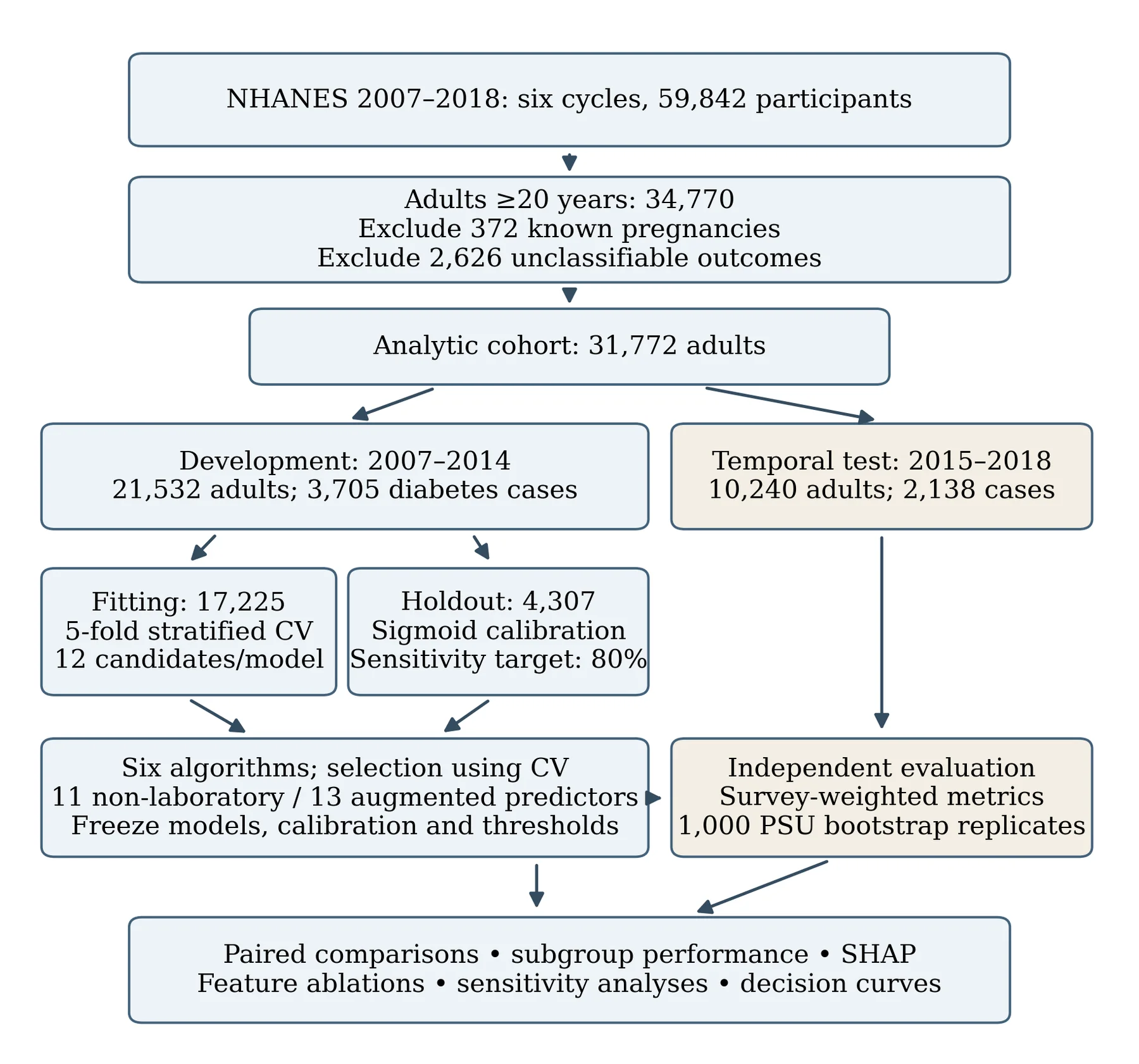
Counts are unweighted. CV denotes cross-validation; PSU denotes primary sampling unit. The temporal test was excluded from fitting, calibration, threshold selection, and algorithm selection.
3.2 Outcome definition and leakage prevention
A binary outcome was defined as positive if the participant reported the doctor diagnosed diabetes, current insulin use, current oral diabetes medication use, or HbA1c ≥6.5%. This is the same as diagnostic advice; however, a single abnormal research measurement is not a clinically confirmed diagnosis [3]. No attempt was made to differentiate the type of diabetes. Negative classification was defined as a valid response of “no” or “borderline” to diagnosis and an HbA1c of < 6.5% without an explicit “yes” medication answer. Responses of "not applicable" were used for missing medications where they were compatible with the questionnaire skip pattern for those who were not diagnosed positive. The ambiguous target outcome records were not included and were not classified to the negative class.
Prediabetes still came up in the negative class, according to the primary definition of diabetes. HbA1c, glucose, self-reported diabetes diagnosis, and diabetes medication variables were only used to create the outcome or create a sensitivity cohort. They did not predict. Participant identifiers, survey cycle, weights, strata, and PSU identifiers were also excluded from the predictor matrix. This separation means that it is not possible to directly reconstruct the target based on its defining variables. It is not a measure of reverse causality; body measures and lipid values may be a result of the prior disease or treatment being given and thus may not be a valid measure of disease prevalence.
3.3 Predictor scenarios and preprocessing
For the non-laboratory scenario, there were 11 predictors: age, BMI, waist circumference, mean systolic and diastolic blood pressure, household income-to-poverty ratio, recorded sex, race/ethnicity, education, smoking status, and a physical-activity indicator. HDL cholesterol and total cholesterol were added to the laboratory-augmented scenario (13 predictors). The same participants and partitions were used for the two scenarios. Non-laboratory prediction is not a questionnaire-only approach; it still uses anthropometry and blood-pressure measurement. Age was top-coded at 80 in order to provide top-coding consistency between cycles. Stable broad race/ethnicity categories were taken from RIDRETH1. A variable DID070, which was a proxy for oral medication, was harmonized with DIQ070 in the subsequent years. Smoking responses and lifetime cigarette exposure were combined.
Physical activity was self-reported moderate or vigorous work or leisure activity (not meeting activity guidelines). The mean of the first, second, and third blood pressure readings was used. Where applicable, “do not know” and refusal codes were recoded as missing predictor values for the individual survey. Median imputation and normalization were performed on numeric predictors, and mode imputation and one-hot encoding were performed on categorical predictors. The transformations were estimated within each fitting fold, and unseen categories were handled without using the validation information. No target-driven feature selection or synthetic oversampling/class balancing was done. The fixed predictor sets were selected to facilitate interpretation and cross-cycle availability. CatBoost was also given the same one-hot-encoded matrix as the other algorithms; the native ability of CatBoost to handle categorical features was not assessed.
3.4 Development, tuning, and temporal testing
The number of adults in the development population was 21,532 for the years 2007-2014. The outcome-by-cycle stratification split was 17,225 model fits and 4,307 holdouts for an independent development calibration. The temporal test comprised 10,240 adults from 2015 to 2018. A test of performance under temporal population change is preserved by not disturbing the later cycles, which are interpretable. It is not a determination of transportability to another health care system or country. The following models were trained: logistic regression, RBF-kernel support vector machine, random forest, XGBoost, CatBoost, and a multilayer perceptron. These methods include a parametric baseline, a kernel classifier, bagged trees, boosted trees, and a neural-network model [20], [21], [22], [23], [24].
For each model–scenario combination, 12 hyperparameter candidates and 5 stratified cross-validation folds were used, and the mean survey weighted ROC-AUC was used as the selection criterion. The random seeds became fixed to 20261007. The development CV was used to select the best algorithm for each scenario prior to the temporal-test evaluation. The hyperparameters used are shown in Appendix Table A1. CV values were used for tuning and model selection and not nested-CV or optimism-corrected estimates of internal performance. No separate full-pipeline bootstrap of the development of the model was done. A model-specific sample-size calculation was not used, and all available observations with meeting criteria were used in the study. Sample size is not enough to determine adequacy for flexible models [25], as event numbers were large.
3.5 Survey weights and calibration
The weights used in the four development cycles and two temporal test cycles were reduced by half in the mobile examination center. Survey weights were normalized to be of mean one in the fitting population. It was found that the preprocessing transformations themselves were not weighted. But weighted evaluation estimates pertain to the eligible population represented by the examination sample, subject to outcome nonresponse and other exclusions. No weighting for item nonresponse was done. A sigmoid calibration model was fitted on the independent development holdout for each hyperparameter chosen. If the decision score of the classifier is available, it was used as its input; otherwise, the logit of the raw predicted probability. Fitted base model was not later used to refit with calibration participants. This was denoted by s and was written as Equation 1.
p_i = 1 / (1 + exp{−(a + bs_i)}) (1)
Weighted logistic regression was used to estimate parameters a and b in the calibration holdout. The classification threshold was the highest threshold that would give at least 80% weighted sensitivity in that holdout, and then it was fixed. Calibration/operating-point selection was the same as that of the same holdout, and the nominal 80% represents a development target and is not an unbiased performance estimate nor an assurance of sensitivity for temporal tests.
Temporal calibration was evaluated using calibration-in-the-large (a calibration slope and intercept jointly estimated) and probability-bin plots. The predicted logit was the offset for the calibration-in-the-large intercept; the ideal value for the intercept is zero. The estimated slope is equal to one, which is an ideal value. The Brier score was used to summarize the squared probability error, which is in Equation 2 [6], [15], [16].
BS_w = (∑_{i = 1}^{n}w_i(y_i − p_i)^2) / (∑_{i = 1}^{n}w_i) (2)
In Equation 2, wᵢ is the examination weight, yᵢ is the binary outcome, and pᵢ is the predicted probability. Lower values indicate better overall probability accuracy; the score reflects both discrimination and calibration and depends on outcome prevalence.
3.6 Performance metrics and statistical comparisons
The main discrimination metric used was survey-weighted ROC-AUC. The precision–recall performance was measured as average precision, rather than trapezoidal integration of the precision–recall curve. Average precision can be used in conjunction with ROC-AUC when positive response is relatively rare [26]. Sensitivity, specificity, F1 score, and Matthews correlation coefficient, as well as accuracy and Brier score, were also determined. For the thresholds depending on the thresholds, the frozen threshold value was used. Matthews correlation coefficient combines all four parts of the confusion matrix and provides more information than accuracy and F1 score [27]. Within public masked strata [28], 1,000 Rao–Wu rescaled PSU bootstrap replications were used to estimate uncertainty. The strata and PSUs were originally specified in the temporal-test design roster, which included PSUs that did not contain any members of a given analytic group.
Of the m PSUs in a stratum, m−1 PSUs were sampled with replacement, and the weight of each PSU was multiplied by m/(m−1) times the number of times the PSU was sampled. The weights of all models were the same, and thus paired comparisons were preserved. Approximate t-based Wald intervals were based on bootstrap standard errors and 30 survey design degrees of freedom. Intervals of bounded metrics were limited to their natural ranges. These intervals are conditional on the models that have been fit and are measures of uncertainty in test-population sampling, not of uncertainty in the processes of model development. In the feature scenario of each of the nonlinear models, the model was compared to logistic regression.
In each scenario the 5 ROC-AUC comparisons were controlled for multiplicity by Holm adjustment [29]. A different family made comparisons between laboratory-enhanced and non-laboratory AUC for every algorithm. 95% intervals for each individual have not been adjusted for simultaneous coverage. As supplementary analyses, ordinary paired DeLong tests were computed but were not used to adjust primary survey-aware results, as their independence assumptions did not address NHANES clustering.
3.7 Subgroups, ablations, and sensitivity analyses
The main discrimination metric used was survey-weighted ROC-AUC. The precision–recall performance was measured as average precision, rather than trapezoidal integration of the precision–recall curve. Average precision can be used in conjunction with ROC-AUC when positive response is relatively rare [26]. Sensitivity, specificity, F1 score, and Matthews correlation coefficient, as well as accuracy and Brier score, were also determined. For the thresholds depending on the thresholds, the frozen threshold value was used. Matthews correlation coefficient combines all four parts of the confusion matrix and provides more information than accuracy and F1 score [27]. Within public masked strata [28], 1,000 Rao–Wu rescaled PSU bootstrap replications were used to estimate uncertainty. The strata and PSUs were originally specified in the temporal-test design roster, which included PSUs that did not contain any members of a given analytic group.
Of the m PSUs in a stratum, m−1 PSUs were sampled with replacement, and the weight of each PSU was multiplied by m/(m−1) times the number of times the PSU was sampled. The weights of all models were the same, and thus paired comparisons were preserved. Approximate t-based Wald intervals were based on bootstrap standard errors and 30 survey design degrees of freedom. Intervals of bounded metrics were limited to their natural ranges. These intervals are conditional on the models that have been fit and are measures of uncertainty in test-population sampling, not of uncertainty in the processes of model development. In the feature scenario of each of the nonlinear models, the model was compared to logistic regression.
In each scenario the 5 ROC-AUC comparisons were controlled for multiplicity by Holm adjustment [29]. A different family made comparisons between laboratory-enhanced and non-laboratory AUC for every algorithm. 95% intervals for each individual have not been adjusted for simultaneous coverage. As supplementary analyses, ordinary paired DeLong tests were computed but were not used to adjust primary survey-aware results, as their independence assumptions did not address NHANES clustering.
3.8 Explainability, decision curves, and reproducibility
The probability of the final calibration was explained using the permutation SHAP applied to the frozen laboratory-augmented winner, including preprocessing [31]. A total of 60 background and 150 temporal-test participants were sampled, from the development fitting partition, with probabilities proportional to survey weights, and from the temporal-test partition, uniformly for explanation. Independent masking and five permutation cycles were used. The resulting importance summaries represent the importance of that sample, not of a population-weighted causal effect. Correlated predictors may be attributed to the same predictor, and independently masked combinations may not represent realistic people. The explanation was approached as an audit of the predictions, rather than a replacement for validation [32]. Two scenario winners were compared to screening everyone or no one over thresholds of 0.05–0.40 using exploratory decision-curve analysis. The weighted net benefit was determined by Equation 3 [33].
NB(t) = TP_w / W − FP_w / W × t / (1 − t) (3)
Here, TPw and FPw are weighted true-positive and false-positive totals, W is the total weight, and t is the threshold probability. The ratio t/(1−t) expresses the assumed relative penalty of a false-positive decision. This analysis did not incorporate local testing costs, capacity, treatment effects, or prospectively elicited preferences.
The supplied research run used Python 3.11.5, scikit-learn 1.8.0, XGBoost 3.2.0, CatBoost 1.2.10, and SHAP 0.51.0. Audit records included download URLs and hashes, cohort membership, partition assignments, CV results, selected configurations, and participant-level probabilities. Reported AUC, average precision, Brier score, sensitivity, and specificity were independently reproduced from all 12 temporal prediction files before manuscript preparation. Model coefficients and estimators were not retuned during that verification.
4 Results
4.1 Participants and data completeness
The final cohort included 31,772 adults with 5,843 adults having diabetes. In the development set, 3,705 cases were observed in 21,532 adults and in the temporal test set, 2,138 cases were observed in 10,240 adults. Table 1 presents unweighted counts and characteristics for the two time periods. The unweighted diabetes fraction in the test sample was 20.9%, while the survey-weighted diabetes fraction was 14.8%. This discrepancy illustrates the fact that sample proportions and population-weighted evaluation should not be given the same meaning.
The retained samples numbered 5,389, 5,743, 5,031, 5,369, 5,202, and 5,038 across the six consecutive cycles. Weighted diabetes prevalence ranged from 11.7% to 12.8% during development and was 14.4% in 2015–2016 and 15.1% in 2017–2018. The highest rates of missingness for a predictor in any cycle were for income-to-poverty ratio in 2017–2018 (13.2%). Predictors were imputed within training folds, and exclusion was used for outcome uncertainty. These various missing data mechanisms have different implications: If imputation is performed, predictor-incomplete participants remain in the analysis, but if outcome-incomplete participants are excluded, the target population may be changed.
Table 1. Development and temporal-test cohort characteristics.
| Characteristic | Development 2007–2014 | Temporal test 2015–2018 |
|---|---|---|
| Participants, | 21,532 | 10,240 |
| Diabetes cases, n | 3,705 | 2,138 |
| Diabetes, unweighted % | 17.2 | 20.9 |
| Diabetes, weighted % | 12.2 | 14.8 |
| Age, years | 47.5 (16.8) | 48.6 (17.2) |
| BMI, kg/m² | 28.8 (6.8) | 29.6 (7.1) |
| Waist circumference, cm | 98.7 (16.3) | 100.7 (17.0) |
| Systolic BP, mmHg | 121.7 (17.1) | 123.9 (17.6) |
| Diastolic BP, mmHg | 70.4 (12.1) | 71.4 (11.9) |
| Female, weighted % | 51.4 | 51.4 |
Figure 2 displays predictor missingness before imputation in the classifiable analytic cohort. Missingness was highest for the income-to-poverty ratio in 2017–2018 (13.2%), while age, sex, and race/ethnicity were complete. The common color scale spans 0–100%, so modest missingness appears pale and should not be interpreted as complete availability. Variation by cycle supports retaining fold-specific imputation and reporting the availability of each predictor.
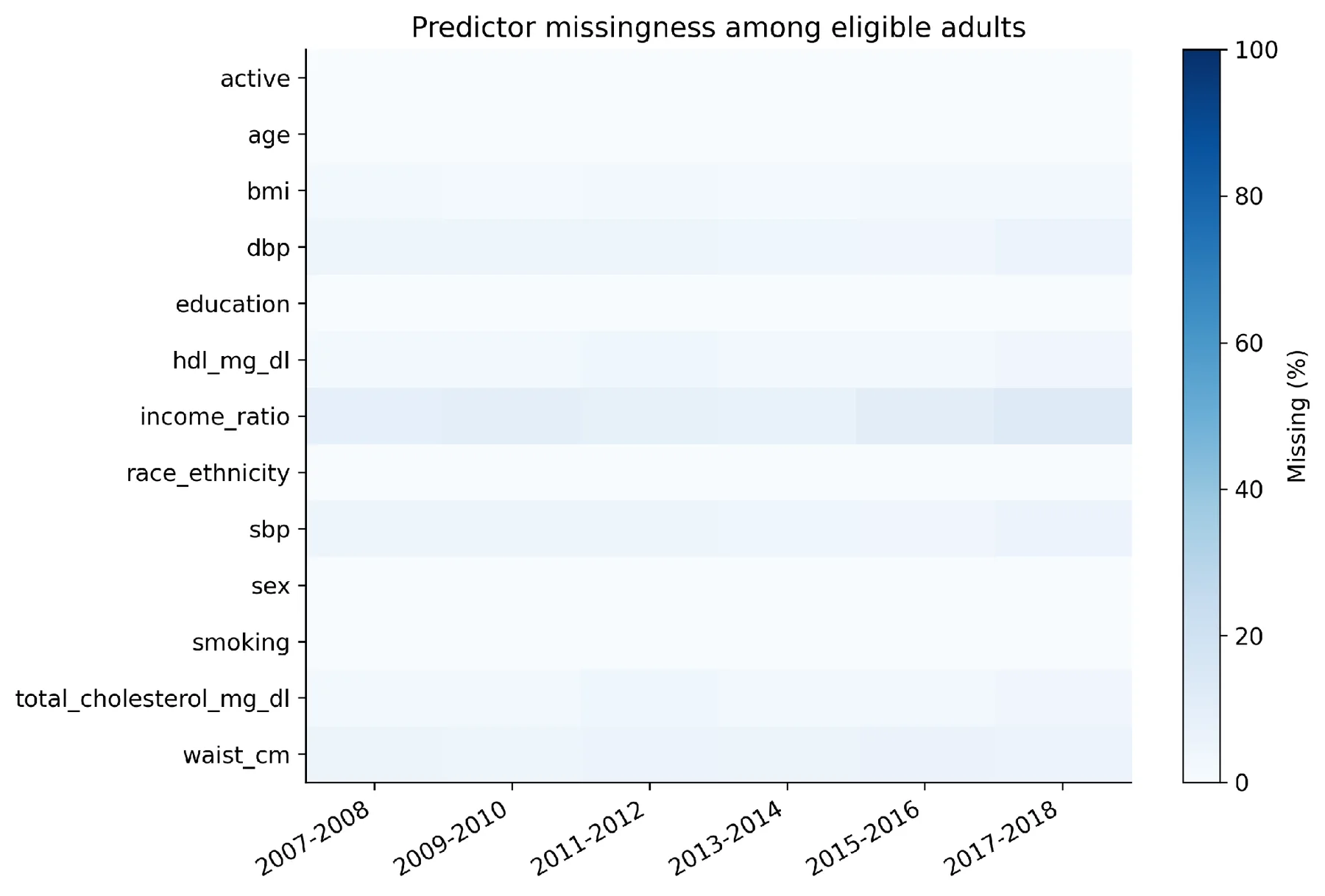
The percentages of cells with missing values before imputation, by feature and cycle, are shown. BMI is body mass index; sbp and dbp are systolic and diastolic blood pressure; income_ratio is family income-to-poverty ratio; race_ethnicity and education are coded demographic characteristics; active is taking moderate to vigorous activity; hdl_mg_dl and total_cholesterol_mg_dl are lipid levels in mg/dL.
4.2 Model selection and temporal discrimination
The development tuning AUCs for CatBoost in both cases (without laboratory variables and with lipid augmentation) were the highest (0.8356 and 0.8569, respectively). Therefore, it was chosen prior to temporal testing. These later-period AUCs were 0.8090 and 0.8362. The above difference between these CV values and the temporal ones is descriptive in nature, as the tuning scores are selection-biased and should not be taken as an unbiased estimate of temporal degradation. All model discrimination and probability values are reported in Table 2. For non-laboratory AUCs, the ones for SVM and CatBoost were 0.7487 and 0.8090, respectively. Logistic regression got the lowest score at 0.8036, whereas the three top alternatives—CatBoost, MLP, and XGBoost—were very close together.
Laboratory augmentation resulted in higher discrimination for all the algorithms. CatBoost achieved AUC 0.8362 (95% CI 0.8206–0.8517), followed numerically by XGBoost (0.8354), MLP (0.8350), and random forest (0.8335). These close estimates do not prove that CatBoost outperforms those three models, as the prespecified inferential comparisons of CatBoost were performed only with logistic regression, not with any combination of pairs of models, except the comparison with logistic regression. The results of the non-laboratory and laboratory-augmented scenarios are shown in the ROC and precision–recall curves in Figures 3 and 4, respectively. The curves for the laboratory augmented models are generally higher, and both the tree and MLP curves are fairly similar. CatBoost average precision went up from 0.3961 without laboratory predictors to 0.4646 with lipid measures (95% CI 0.4354–0.4939).
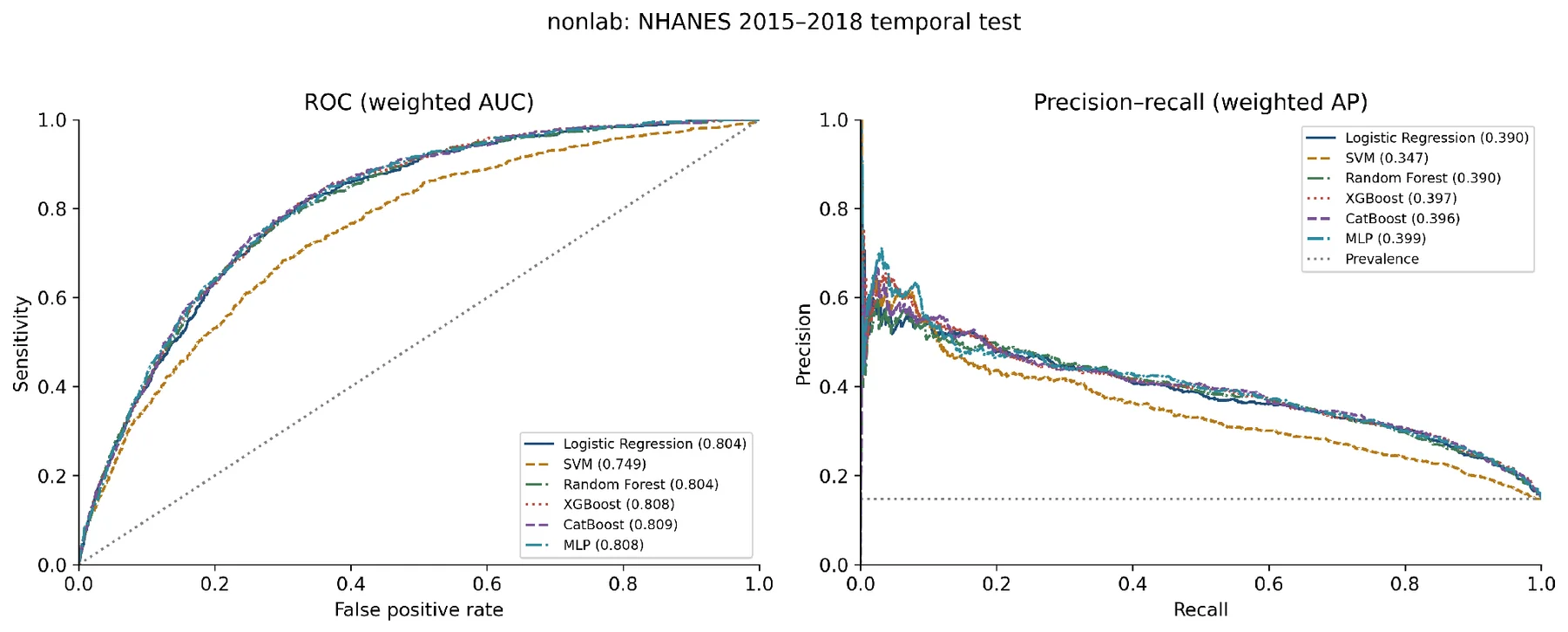
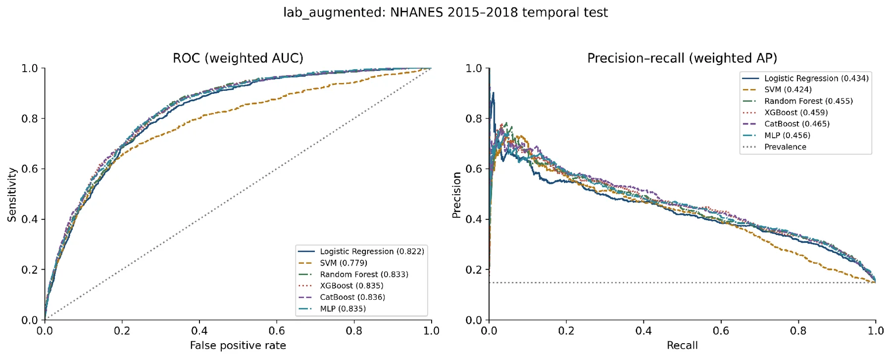
Both are above the precision–recall reference line of the weighted test prevalence of 0.1477. Even their absolute values suggest a significant burden of false-positive results at sensitivity thresholds.
Table 2. Survey-weighted discrimination and probability performance.
| Set | Model | AUC (95% CI) | AP | Brier | CITL | Slope |
|---|---|---|---|---|---|---|
| NL | LR | 0.804 (0.787–0.820) | 0.390 | 0.1070 | 0.027 | 0.875 |
| NL | SVM | 0.749 (0.727–0.770) | 0.347 | 0.1264 | 0.193 | 4965.344 |
| NL | RF | 0.804 (0.787–0.821) | 0.390 | 0.1061 | 0.065 | 0.862 |
| NL | XGBoost | 0.808 (0.792–0.824) | 0.397 | 0.1061 | 0.024 | 0.831 |
| NL | CB | 0.809 (0.793–0.825) | 0.396 | 0.1058 | 0.040 | 0.844 |
| NL | MLP | 0.808 (0.792–0.825) | 0.399 | 0.1053 | 0.050 | 0.857 |
| LA | LR | 0.822 (0.806–0.838) | 0.434 | 0.1029 | 0.050 | 0.895 |
| LA | SVM | 0.779 (0.759–0.799) | 0.424 | 0.1086 | 0.151 | 0.929 |
| LA | RF | 0.833 (0.817–0.850) | 0.455 | 0.1001 | 0.045 | 0.881 |
| LA | XGBoost | 0.835 (0.819–0.851) | 0.459 | 0.0999 | 0.061 | 0.871 |
| LA | CB | 0.836 (0.821–0.852) | 0.465 | 0.0994 | 0.057 | 0.877 |
| LA | MLP | 0.835 (0.819–0.851) | 0.456 | 0.0999 | 0.064 | 0.893 |
AUC confidence intervals use the survey bootstrap. AP is average precision. CITL is calibration-in-the-large; ideal CITL = 0 and slope = 1. NL denotes non-laboratory; LA denotes laboratory-augmented; LR denotes logistic regression; RF denotes random forest; and CB denotes CatBoost.
The left panel shows survey-weighted ROC curves with AUCs in the legend; the right panel shows precision–recall curves with average precision (AP). The ROC diagonal denotes chance ranking. The horizontal precision–recall reference represents the weighted diabetes prevalence of 0.1477. All six models use the same temporal-test participants.
The left and right panels show survey-weighted ROC and precision–recall curves, respectively. Legends report AUC and AP. The same temporal-test cohort and reference lines are used as in Figure 3, enabling comparison between feature scenarios. Figure 5 summarizes AUC uncertainty for all six algorithms in both scenarios. The laboratory-augmented estimates are consistently higher, while intervals for the leading nonlinear models overlap substantially. These are intervals for individual AUCs; their overlap does not test a paired difference. The prespecified paired comparisons in Table 3 provide the appropriate inference against logistic regression.
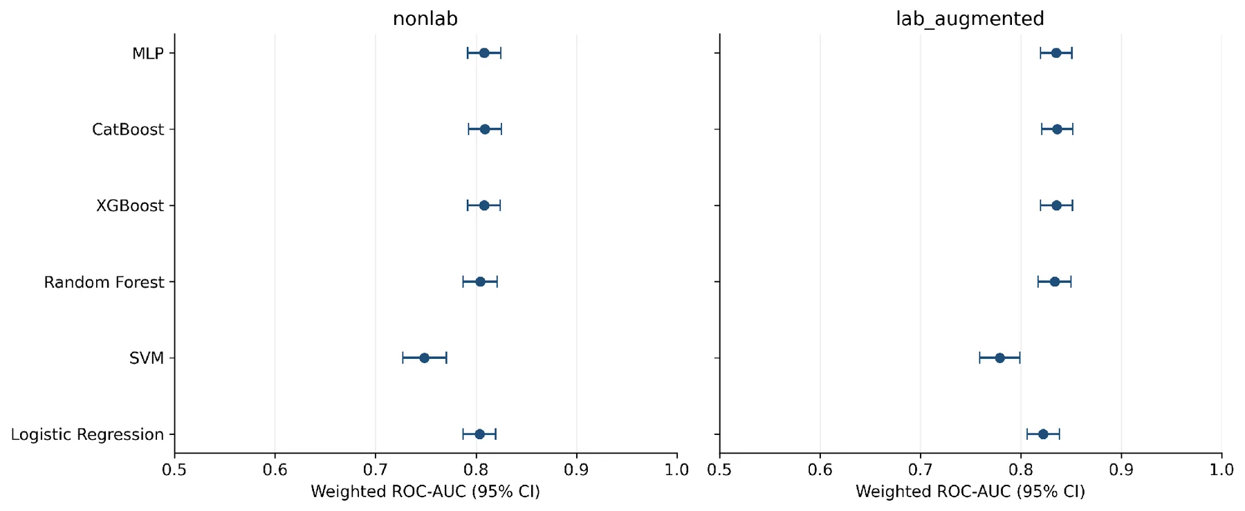
Survey-weighted AUC estimates are represented by points, and individual 95% confidence intervals for AUC are represented by horizontal bars. The panels are the non-laboratory and lab-augmented scenarios. The significance of a paired model comparison is not determined just by interval overlap.
4.3 Paired comparisons and operating characteristics
Survey-aware paired AUC comparisons to logistic regression are shown in Table 3. In the laboratory-augmented scenario, CatBoost improved AUC by 0.0139 (95% CI 0.0081–0.0197; Holm-adjusted p = 0.00012). Random forest, XGBoost, and MLP also outperformed logistic regression when adjusted for. In the non-laboratory scenario, CatBoost’s AUC difference was 0.0054 (95% CI 0.0004–0.0104), but its adjusted p value was 0.138. The unadjusted interval, including zero and the adjusted test that is not significant can be reconciled, as the interval is not simultaneous. None of the nonlinear models considered, apart from logistic regression, showed an adjusted significant improvement. Within CatBoost, adding lipid measures increased AUC by 0.0271 (95% CI 0.0181–0.0362; adjusted p < 0.00001). Increments were 0.0187 for logistic regression, 0.0302 for SVM, 0.0293 for random forest, 0.0274 for XGBoost, and 0.0267 for MLP, with all six within-algorithm comparisons remaining significant after adjustment. The increase from extra data, provided by CatBoost, was numerically greater than the increase it provided when it was enhanced with the laboratory. This is a descriptive comparison between effect sizes—not a separate statistical test comparing those increments.
Table 3. Paired survey-weighted AUC differences from logistic regression.
| Set | Model | AUC difference (95% CI) | Adjusted p |
|---|---|---|---|
| NL | SVM | -0.0549 (-0.0708 to -0.0389) | <0.00001 |
| NL | RF | 0.0006 (-0.0062 to 0.0074) | 0.85817 |
| NL | XGBoost | 0.0044 (-0.0004 to 0.0092) | 0.21416 |
| NL | CB | 0.0054 (0.0004 to 0.0104) | 0.13764 |
| NL | MLP | 0.0047 (-0.0009 to 0.0103) | 0.21416 |
| LA | SVM | -0.0433 (-0.0569 to -0.0297) | <0.00001 |
| LA | RF | 0.0112 (0.0036 to 0.0188) | 0.00515 |
| LA | XGBoost | 0.0131 (0.0070 to 0.0192) | 0.00039 |
| LA | CB | 0.0139 (0.0081 to 0.0197) | 0.00012 |
| LA | MLP | 0.0127 (0.0066 to 0.0188) | 0.00039 |
Differences are the specified model—logistic regression—in the same scenario. Confidence intervals are done one at a time, 95% intervals. Holm-adjusted p-values are for the 5 models versus LR tests in each scenario. In both cases, SVM was less accurate.
Table 4 provides threshold-dependent metrics. Laboratory-augmented CatBoost used a frozen probability threshold of 0.13946 and achieved sensitivity of 77.9% (95% CI 75.0–80.9%), specificity of 74.4% (72.3–76.4%), F1 of 0.4783, MCC of 0.3935, and accuracy of 74.9%. The non-laboratory one obtained a sensitivity of 77.6% and a specificity of 70.6%. These results are at the target operating point for intended sensitivity; thus, any accuracy comparison should be made with caution using an unqualified 0.5 threshold. The classification trade-offs of all six models are plotted at their respective frozen development thresholds in figures 6 and 7. Lipid augmentation resulted in a decrease in the weighted false-positive fraction among non-cases from 29.4% to 25.6% and a decrease of the false-negative fraction from 22.4% to 22.1% for CatBoost. Laboratory-augmented logistic regression outperformed CatBoost in terms of sensitivity (80.0% vs 77.9%) but was inferior to CatBoost in terms of specificity (69.8% vs 74.4%). In both the situations, SVM showed the highest false-positive fractions (47.5% and 43.8%). The weighted percentages in the cells are not numbers of participants but percentages from the observed outcome classes; the thresholds that are printed above the panels are rounded.
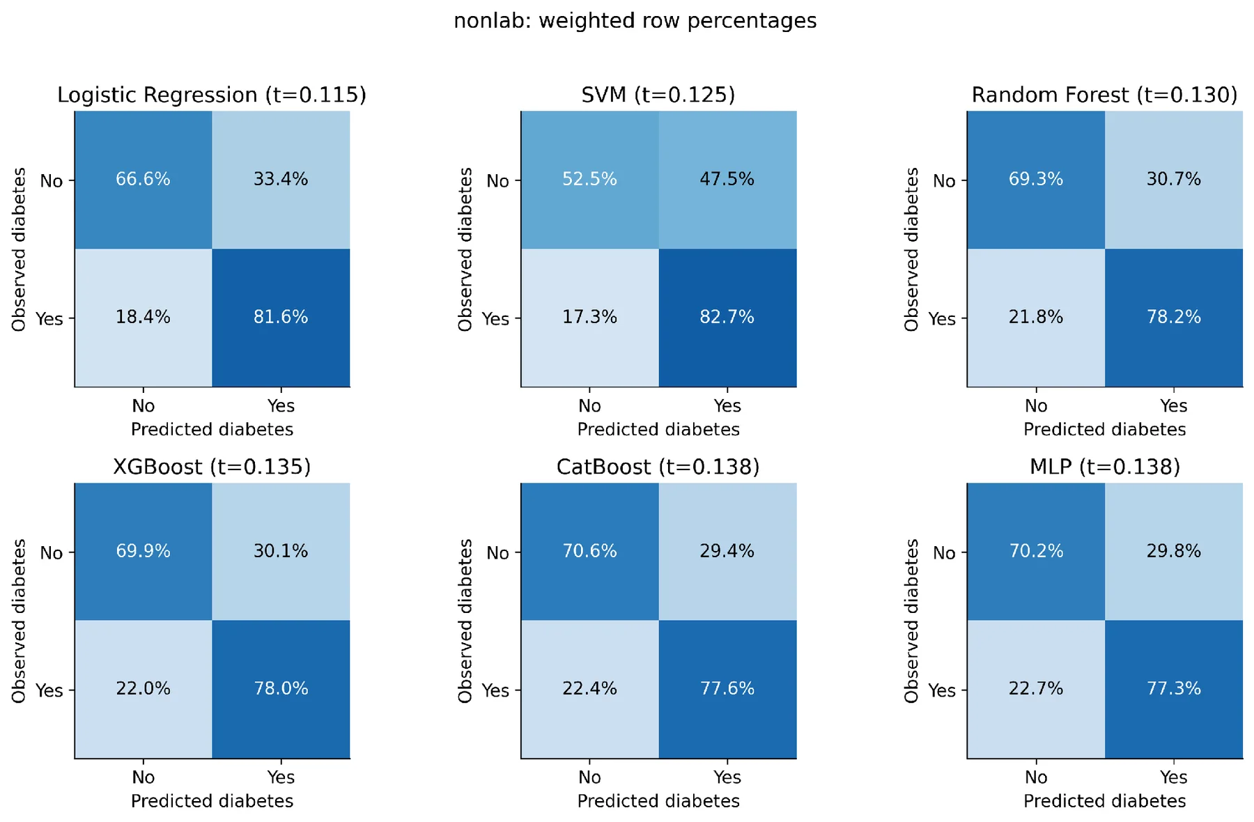
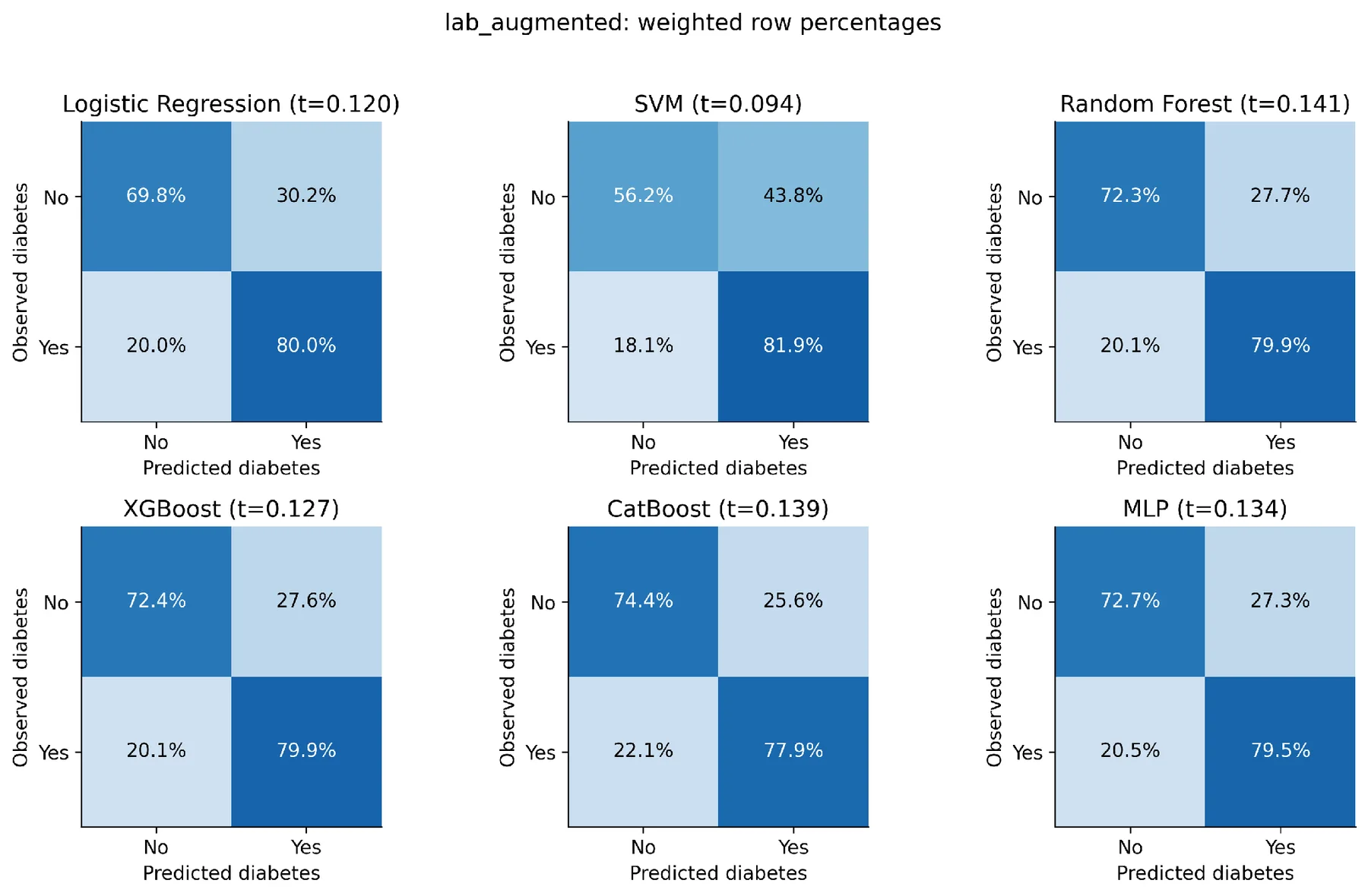
Table 4. Operating characteristics at frozen development thresholds.
| Set | Model | Sensitivity % | Specificity % | F1 | MCC | Accuracy % |
|---|---|---|---|---|---|---|
| NL | LR | 81.6 | 66.6 | 0.436 | 0.348 | 68.8 |
| NL | SVM | 82.7 | 52.5 | 0.362 | 0.250 | 57.0 |
| NL | RF | 78.2 | 69.3 | 0.440 | 0.348 | 70.6 |
| NL | XGBoost | 78.0 | 69.9 | 0.444 | 0.352 | 71.1 |
| NL | CB | 77.6 | 70.6 | 0.447 | 0.356 | 71.7 |
| NL | MLP | 77.3 | 70.2 | 0.443 | 0.350 | 71.3 |
| LA | LR | 80.0 | 69.8 | 0.452 | 0.365 | 71.3 |
| LA | SVM | 81.9 | 56.2 | 0.376 | 0.270 | 60.0 |
| LA | RF | 79.9 | 72.3 | 0.470 | 0.387 | 73.4 |
| LA | XGBoost | 79.9 | 72.4 | 0.471 | 0.388 | 73.5 |
| LA | CB | 77.9 | 74.4 | 0.478 | 0.394 | 74.9 |
| LA | MLP | 79.5 | 72.7 | 0.472 | 0.389 | 73.7 |
Sensitivity, specificity, and accuracy are percentages; F1 and MCC are unitless. Each model’s threshold was chosen only in the development calibration holdout to target at least 80% weighted sensitivity. No temporal-test or subgroup-specific threshold tuning was performed.
Each panel shows one model at its frozen development threshold, rounded to three decimals in the panel title. Rows are observed classes, and columns are predicted classes, with "Yes" indicating diabetes. Cells are survey-weighted row percentages: specificity and false-positive percentage on the upper row, and false-negative percentage and sensitivity on the lower row.
Panels use each model’s frozen development threshold and the same class orientation as Figure 6. Values are survey-weighted percentages within observed outcome classes. They are not raw counts, and their denominators differ between the upper and lower rows. The full-precision thresholds were used to compute Table 4.
4.4 Calibration and the SVM probability anomaly
The Brier score for laboratory-augmented CatBoost was 0.0994 (95% CI 0.0915–0.1073) vs 0.1029 for laboratory-augmented logistic regression. The intercept of its calibration-in-the-large was 0.0565, and the slope was 0.8770. The positive intercept value means that there was a small amount of underprediction and that the slopes below 1 mean that the spread of the predictions was too wide relative to the spread of the outcome gradients. Figure 8 and Figure 9 display deviations from the ideal calibration line, especially when the predicted probability is high. The bins plotted are descriptive, and no confidence bands were estimated.
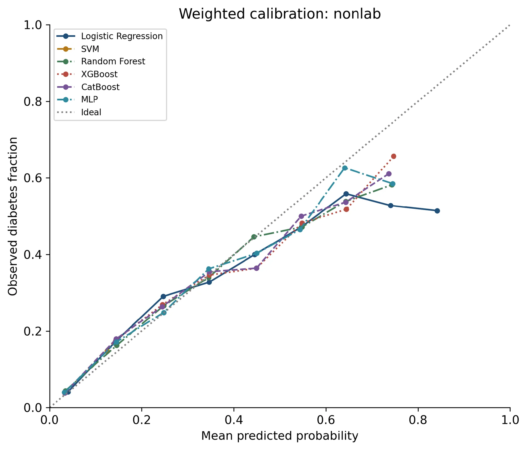
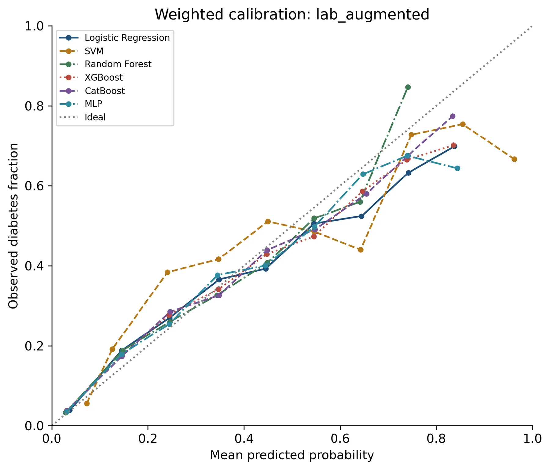
Probability performance in time did not consistently benefit from development based sigmoid calibration. For CatBoost with Lab, the raw Brier score was 0.09928, the raw calibration slope was 0.9586, the calibrated Brier score was 0.09938, and calibrated calibration slope was: 0.8770. Calibration in large was improved from 0.1363 to 0.0565. So, although the average calibration improved, there was a less favorable slope and a slightly higher Brier score. MLP exhibited a slight Brier improvement while a few of the tree-model Briers were either flat or slightly higher. The untested differences should not be called a statistically proven improvement or harm.
The non-laboratory SVM had to be looked at on its own. Its saved probabilities were between 0.124918 and 0.125191; the standard deviation was ~0.000021. The estimated calibration slope was almost zero (4,965.34) and is not considered to be acceptable calibration. The probability differences were very small, and its ranking AUC did not change to 0.7487. This comparator thus offers evidence on the ranking performance of the fitted pipeline, rather than on an absolute-risk estimator that can be relied upon. The outlier data were carried over and reported; no test-based correction was used. The archive does not determine if the compression was primarily in the base decision scores, sigmoid optimization, or in the combination of these two.
Values represent the difference between mean predicted probability and the survey-weighted diabetes fraction in the fixed bins (0.1 width). Bins with less than 30 participants are not plotted; lines connect plotted bins. The ideal calibration is indicated by the dotted diagonal. The trace of SVM probabilities are not able to prove calibration on the useful range of probabilities, as the probabilities are focused near 0.125.
Axes, binning, and minimum bin size are done for Figure 8. The points corresponding to underprediction in a bin are above the dotted diagonal, and those corresponding to overprediction are below the dotted diagonal. Descriptive summaries with no uncertainty bands are connected, and differences in bins with high probabilities should not be interpreted as accurate estimates of single bin risks.
4.5 Subgroup and cycle-specific performance
The subgroup AUCs for laboratory-augmented CatBoost are shown in Figure 10. The discrimination was fairly comparable for both sexes, with AUC=0.8316 for males and AUC=0.8396 for females. Subgroup estimates demonstrated a sensitivity of 78.9% and specificity of 71.6% in men and a sensitivity and specificity of 76.9% in women, respectively. All of the following operating metrics are described here independently from the AUC-only figure. Descriptive differences are not on their own evidence of equivalence or inequity and were not submitted to a formal interaction test. Among adults aged 20–44, AUC was 0.8040, yet sensitivity at the common threshold was only 38.6% (95% CI 32.7–44.5%), with specificity 93.8%. In those aged at least 65, sensitivity was 89.0% (85.7–92.3%) and specificity 43.6%.
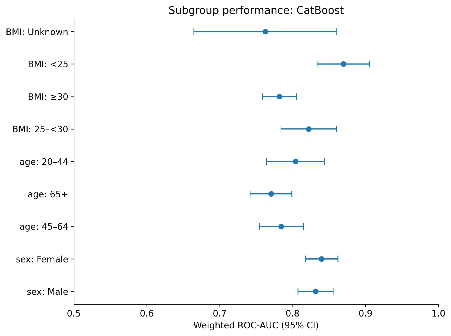
Adults 45-64 years old with sensitivity 80.9% and specificity 63.2%. Thus, the overall sensitivity hides a significant variation in the ratio of missed cases and false positives by age group. Any narrowing of the age-group AUCs should not be interpreted as direct evidence of algorithm failure, and this will also limit between-person variation in a dominant predictor. For BMI < 25 kg/m², AUC was 0.8697, but sensitivity was 55.2%; for BMI ≥ 30 kg/m², AUC was 0.7820 and sensitivity was 85.5%. The missing-BMI group comprised 215 participants and 126 cases and had broad intervals, such as AUC 0.7627 (95% CI 0.6647-0.8606). This group is not to be discarded because its composition reflects the fact that in the absence of measurement, there may be a separate risk profile.
Separate-cycle AUCs were 0.8340 in 2015–2016 and 0.8383 in 2017–2018. They are numerically similar, and there is only limited descriptive stability within the temporal test period (no equivalence test was conducted).
Laboratory-augmented model survey-weighted AUCs and individual 95% survey-bootstrap confidence intervals are represented by points and horizontal bars, respectively. The figure only shows discrimination, not sensitivity or specificity. BMI is in units of kg/m², the <25 group includes underweight participants. The missing-BMI subgroup is kept, and the uncertainty is significantly higher.
4.6 Feature ablations and sensitivity analyses
The removal of lipid measures resulted in a 0.0271 decrease in the CatBoost AUC, while the removal of BMI and waist circumference resulted in a 0.0208 decrease in the CatBoost AUC (95% CI −0.0296 to −0.0120). In contrast, removing smoking and activity changed AUC by only −0.0002 (95% CI −0.0018 to 0.0014). These paired differences are given in Table 5 and Figure 11. Lipid and anthropometric data thus contributed detectably to the chosen configuration. The small lifestyle ablation effect is not to say that smoking or activity is not biologically important; the variables were crude, cross-sectional, and likely to be redundant with other predictors.
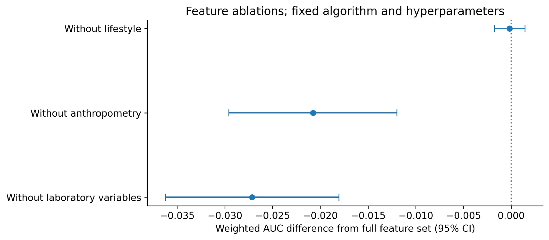
Table 5. CatBoost feature-group ablation results.
| Feature configuration | AUC | Difference (95% CI) | Brier |
|---|---|---|---|
| Full feature set | 0.836 | Reference | 0.0994 |
| Without laboratory variables | 0.809 | -0.0271 (-0.0362 to -0.0181) | 0.1058 |
| Without anthropometry | 0.815 | -0.0208 (-0.0296 to -0.0120) | 0.1034 |
| Without lifestyle | 0.836 | -0.0002 (-0.0018 to 0.0014) | 0.0999 |
Reduced models were implemented using the same algorithm and hyperparameters and refitted and recalibrated with development data. The differences are calculated as the reduced-model AUC -- full-model AUC, based on the same 10,240 test participants. Intervals are pairs of survey-bootstrap 95% intervals.
AUC is full laboratory-augmented CatBoost AUC—paired 95% survey-bootstrap intervals are shown as bars, and points are reduced-model AUC. The vertical dotted line represents no difference. Intervals for lipid and anthropometric removal are below zero, and the lifestyle-removal interval contains zero. For reduced models, hyperparameters were set and models were refitted. Table 6 shows the two sensitivity analyses. The fasting-glucose-inclusive definition retained 4,828 temporal-test participants with 1,136 cases and yielded an AUC of 0.8395 (95% CI 0.8180–0.8611), AP 0.5067, and a Brier score of 0.1070. Due to the different outcome, sample, and weights, the AP or Brier difference is not directly interpretable as an improvement over the primary model. Restricting development to 2011–2014 yielded AUC 0.8328 (95% CI 0.8167–0.8489) on the original test population. These estimates are not to imply that the main discrimination was based solely on the previous cycles, but at the same time the training size was simultaneously altered. Some non-laboratory advantages yielded more apparent evidence with supplementary unweighted DeLong tests, with an adjusted p value of 0.00063 with the CatBoost comparison versus 0.138 with the survey-aware adjusted p value. This discrepancy is a result of various weightings and dependency assumptions and various uncertainty estimates. This main interpretation thus takes the survey-aware analysis over the other approach of choosing the test with the lower p-value.
Table 6. Outcome and historical-cycle sensitivity analyses.
| Analysis | Test | Cases | AUC (95% CI) | AP | Brier |
|---|---|---|---|---|---|
| Primary outcome | 10,240 | 2,138 | 0.836 (0.821–0.852) | 0.465 | 0.0994 |
| Add fasting glucose. | 4,828 | 1,136 | 0.840 (0.818–0.861) | 0.507 | 0.1070 |
| Develop in 2011–2014 | 10,240 | 2,138 | 0.833 (0.817–0.849) | 0.454 | 0.1005 |
All rows use CatBoost. The fasting analysis uses fasting-subsample weights and a different eligible population. The restricted-development analysis uses 2011–2014 for fitting/calibration and the unchanged 2015–2018 primary test set. Confidence intervals are survey-bootstrap intervals.
4.7 SHAP attribution and exploratory net benefit
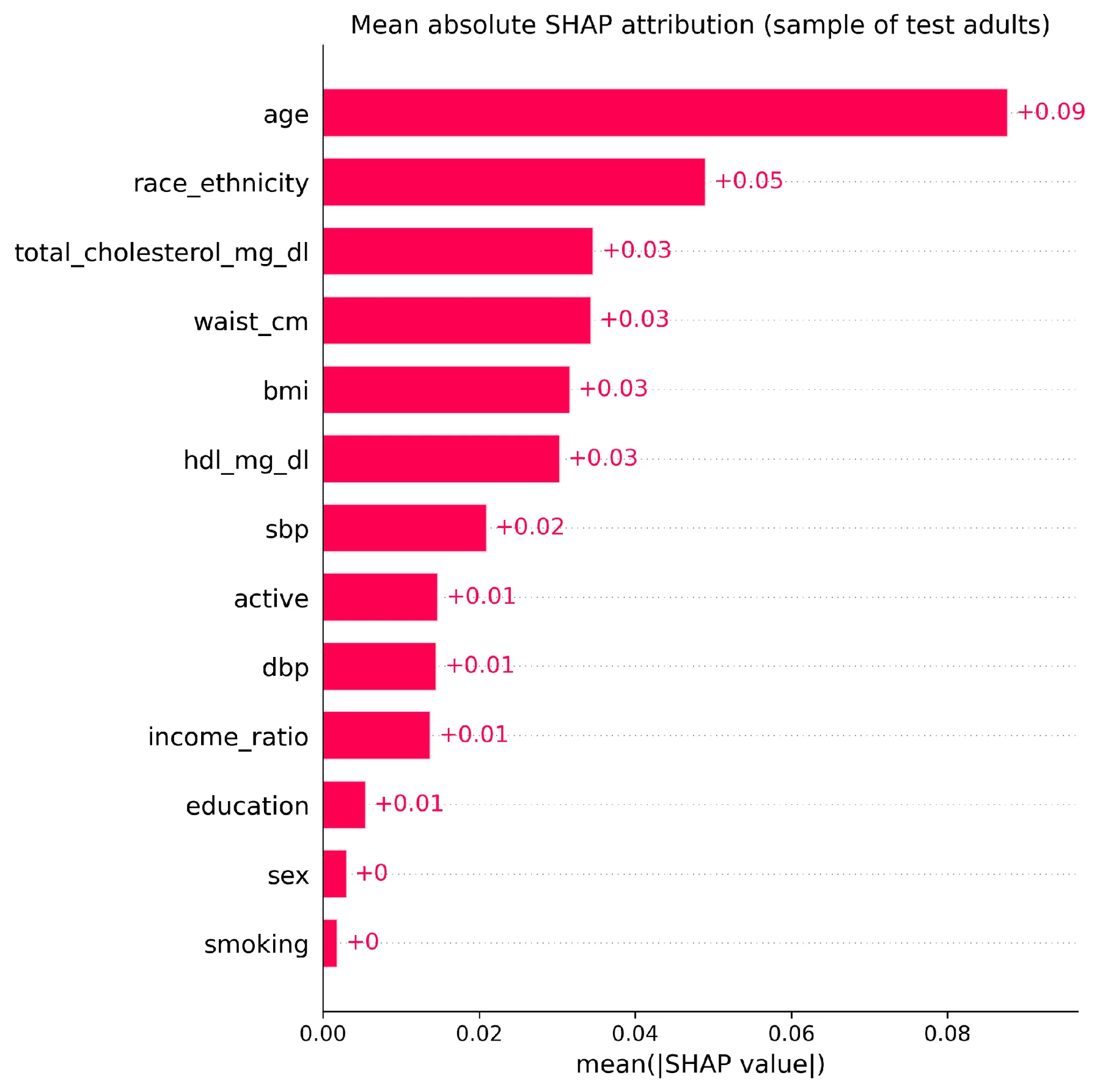
In the 150-participant explanation sample, the top five SHAP contributors were age (0.0877 probability units), race/ethnicity (0.0490), total cholesterol (0.0347), waist circumference (0.0344), BMI (0.0317), and HDL cholesterol (0.0304). The distribution and direction of individual attributions are shown in figure 12, while the ranking of their mean absolute magnitude is shown in figure 13. Waist circumference and BMI were generally associated with predicting a higher value, and higher age also was generally associated with a higher prediction in the plotted sample. Both SHAP and ablation results showed a clear focus on anthropometry measures and lipid measures, which are complementary, indicating that the feature groups were used in the fitted model. SHAP magnitude is not an indication of the direction of an association, and neither SHAP nor an ablation is a causal effect. Race/ethnicity is a general social designation and could also indicate disparities in exposure, diagnosis, treatment, and sampling. The importance of it is not evidence for a biological explanation or justification for clinical deployment without a dedicated equity assessment. The explanation subset is uniformly sampled from the test population, and population level rankings and/or subgroup mechanisms should not be assumed based on these attributions.
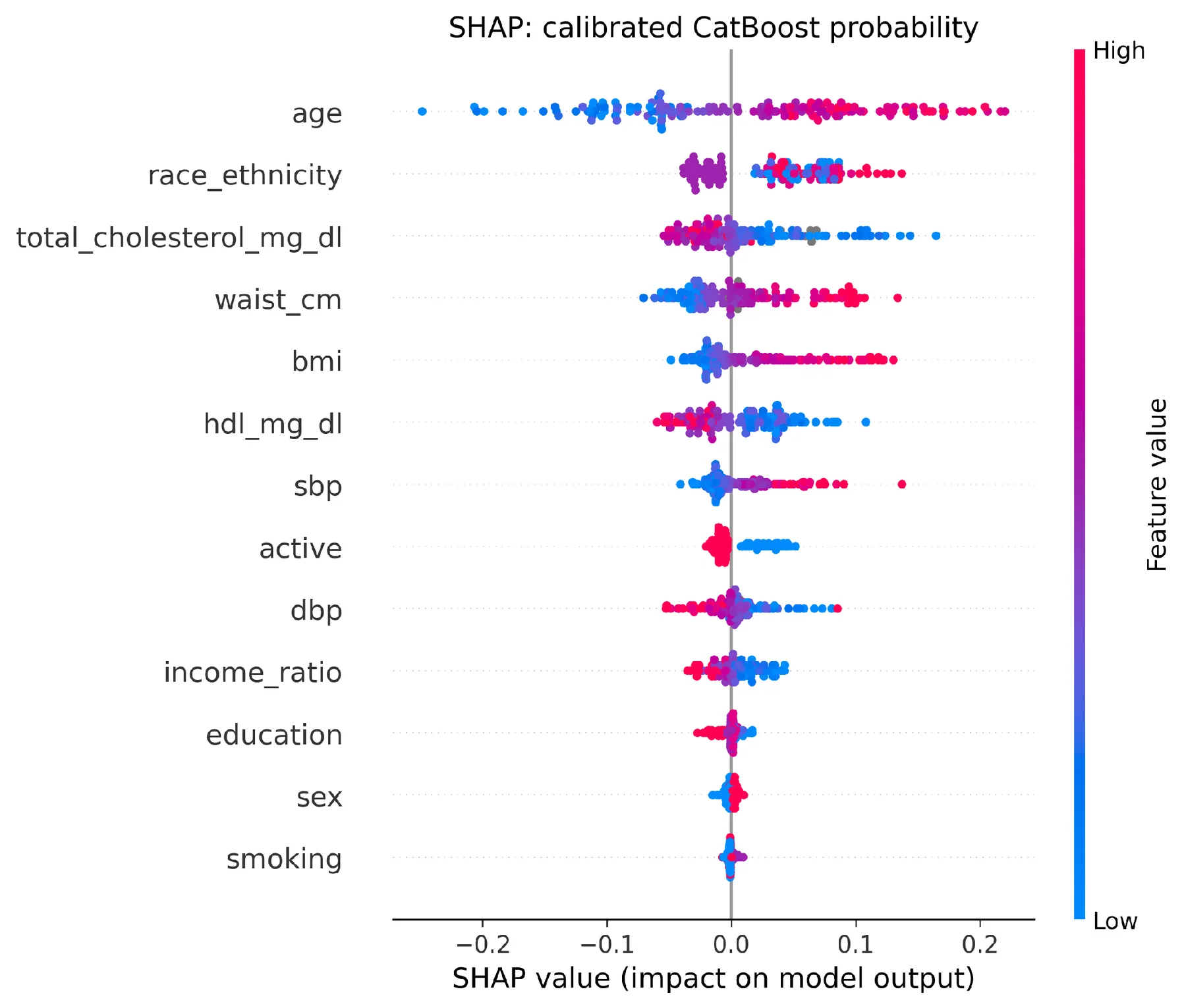
All 150 temporal-test participants are represented by each dot. Positive SHAP values make the calibrated probability higher; negative values make it lower. Color is used to indicate low to high values of the features or numeric codes for categories. Coloring in categorical variables follows the stored numeric code for the variables; there is no clinical order to the nominal coding (e.g., race/ethnicity and sex variables), and no biological or causal interpretation of these numbers is suggested.
Bars represent mean absolute SHAP values, in probability units, for the same 150 participants. The length of the bars does not necessarily reflect a consistent positive relation but rather larger average attribution magnitudes. The rounded labels include a plus sign (+) to indicate that the magnitude is nonnegative (not zero); rounding to +0 does not represent a zero contribution. Figure 14 does not represent a population-average explanation. The background probability was 0.1151, and the contributions added up to a predicted probability of 0.3825. In this example, the HDL cholesterol level of 32 mg/dl was a positive factor, and the race/ethnicity code 1 and age of 53 years, as well as waist circumference of 112 cm, were positive factors, with the blood-pressure values contributing negatively. These directions refer to the fitted model in relation to its background distribution, not that changing a measurement or category would change diabetes occurrence.
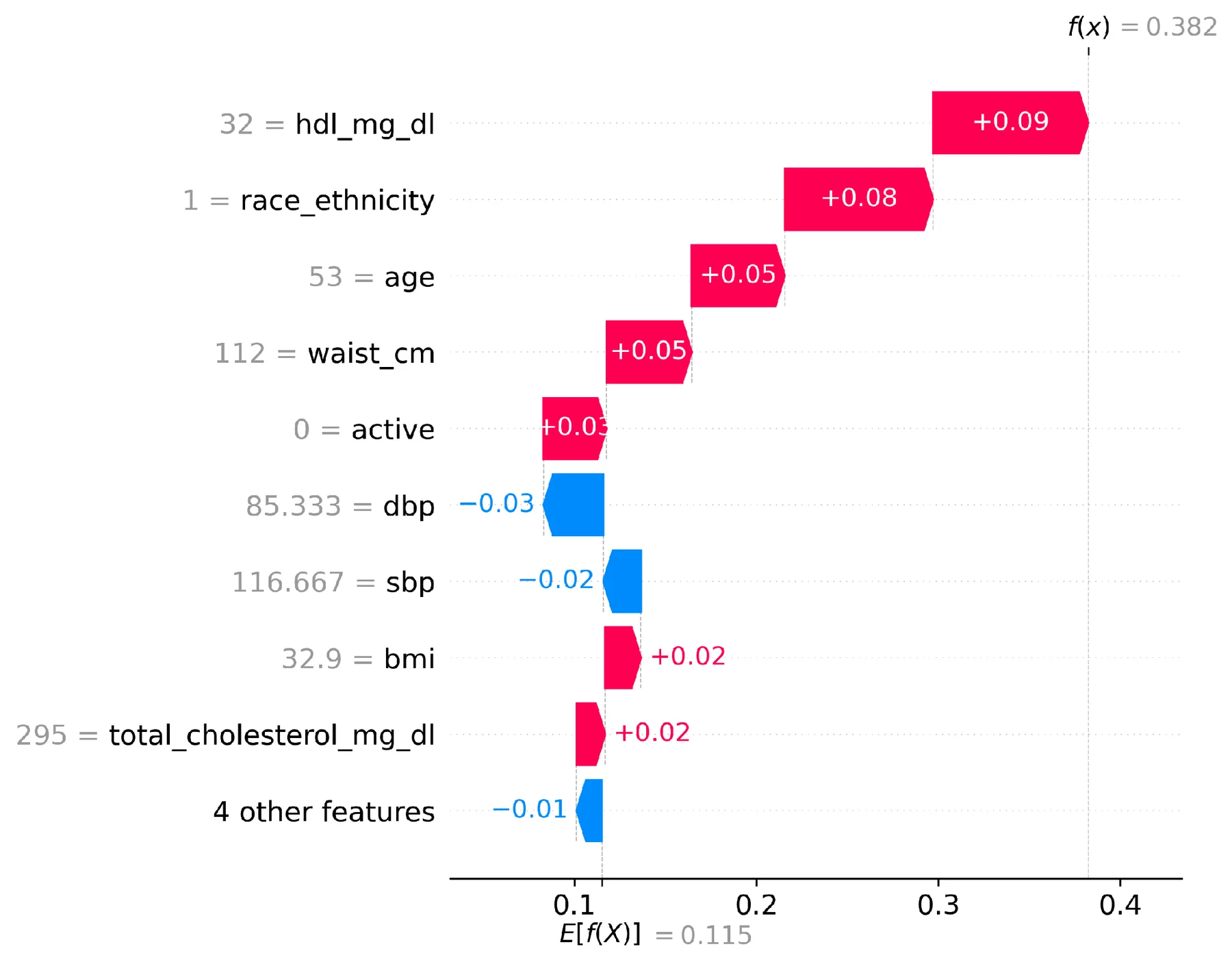
The waterfall begins with the background expectation, E[f(X)], and ends with the participant's calibrated probability, f(x) (values are rounded). Red contributions add more to the prediction, and blue contributions subtract from the prediction. The values of the features exhibited by the participant are shown in the labels; “4 other features” is a group of the four smallest absolute values. This is just for illustrative purposes and not proof of causal effects or representative participants. At all thresholds studied, the laboratory-augmented CatBoost decision curve was generally superior to a screening everyone or a screening no one curve, and both were superior to the non-laboratory curve (Figure 15). This suggests that there is estimated net benefit in this population at the historical level of the threshold-dependent trade-offs. Implementing the curves costs are not included, nor is there evidence that predictions that lead to action will improve health outcomes. The outcome is for people with known diabetes, a screening program would need to identify a separate cohort of people who have not been diagnosed and would need to be evaluated in a prospective fashion.
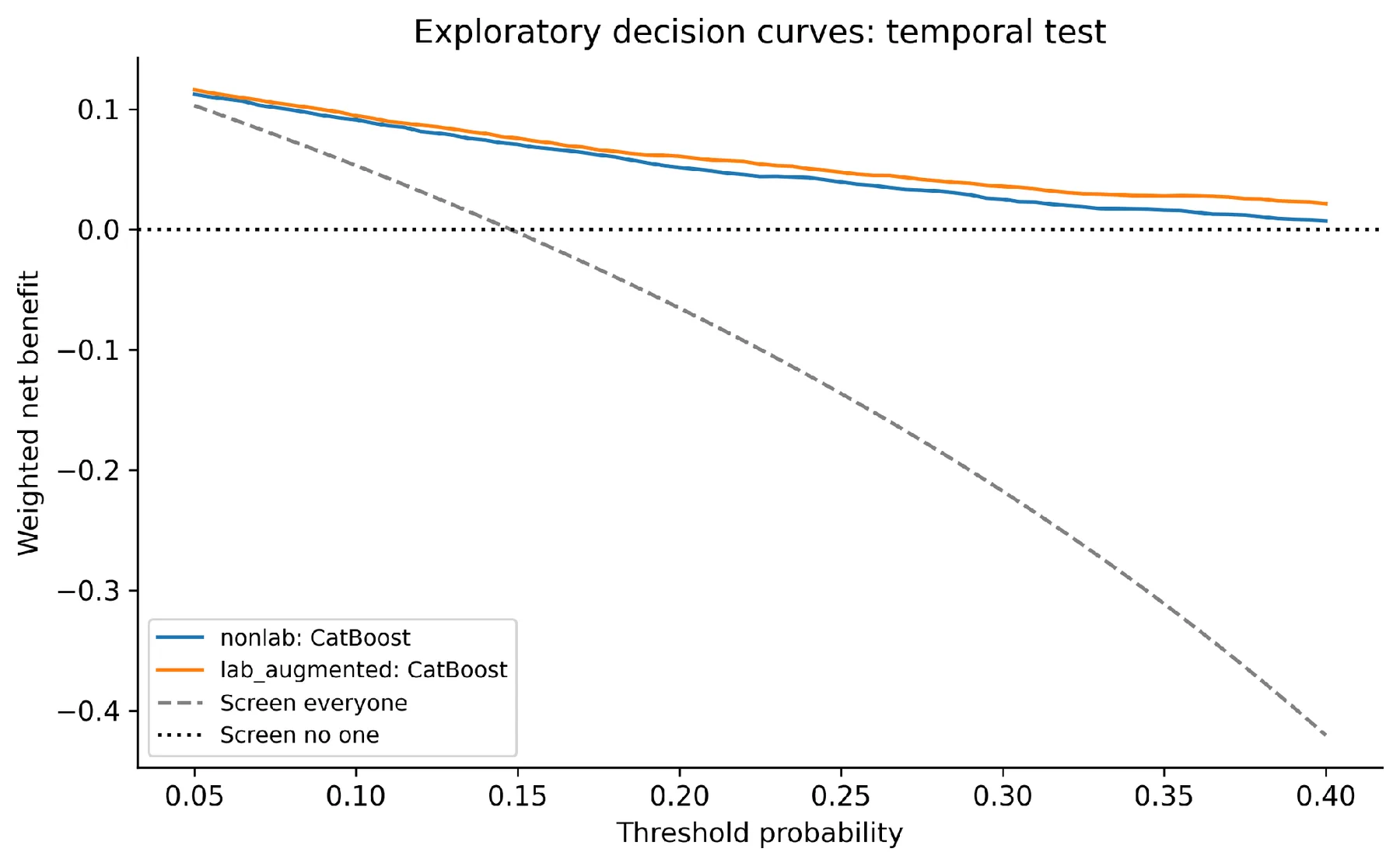
Net benefit is survey-weighted and shown for thresholds 0.05–0.40. Curves compare the two CatBoost feature scenarios with screening everyone or no one. No confidence intervals are shown. The threshold range is exploratory and should not be interpreted as a recommended clinical policy.
5 Discussion
5.1 Main findings and their interpretation
A slight and reproducible benefit of several nonlinear algorithms was observed when the predictors were HDL and total cholesterol. The development-selected winner CatBoost performed the best in terms of temporal AUC, AP, MCC, and Brier score in the laboratory-augmented scenario. It had an AUC of about 1.39 percentage points higher than the logistic regression. However, CatBoost, XGBoost, MLP, and random forest were found to be numerically close and the analysis didn't show that CatBoost is superior to other nonlinear models in a pairwise manner. Algorithmic differences were less without laboratory measurements. When predictor information is limited, it is better to keep an adjusted significant advantage as logistic regression, implying that the more complex baseline should be reserved for more complex situations. This is in line with the general conclusion that prediction is not necessarily better with the increase in model complexity [5]. The matched feature comparison is particularly informative; the CatBoost AUC improvement due to the addition of lipids exceeded what was seen for CatBoost over logistic regression in the lab setting. This indicates that, in this context, the information that a model has at its disposal is at least as important as the selection of competent modelling families.
5.2 Relationship to earlier diabetes prediction studies
An earlier NHANES SVM study had an AUC of 0.835, but used different sets of predictors, outcome rules and validation sets [7]. Then this low SVM performance cannot be generalized to the algorithm in its entirety. Further, the finding of the non-laboratory probability-compression anomaly makes it more difficult to draw conclusions concerning the calibration of that pipeline. Diabetes AUCs in broader NHANES searches have reported much higher values with laboratory inclusion due to different sets of features and case definition and resampling strategies. The current AUC is not a direct copy nor a valid "head-to-head" rejection of those results. The NHANES 2007-2018 comparison, which was based on lifestyle, showed an XGBoost AUC of 0.8168 with significant sensitivity-specificity trade-offs [9].
The present results underscore the importance of being explicit about such trade-offs and introduce a holdout in a later period—survey inferences and lipid ablations. They also demonstrate that an overall sensitivity target is not sufficient to provide sensitivity in younger adults. This is a more targeted contribution than another ranking of an aggregate model. More recent NHANES data, validated against Korean data, have been used in a newer study, which tested the geographic transportability better than the present study on temporal transportability within NHANES [10]. In much the same way, predictor alignment and recalibration can be important components of model assessment when EHRs are being validated against NHANES [14]. These studies suggest the following steps: (1) use models on real-world contemporary data that is independent from the models, (2) assess an undiagnosed population, and (3) investigate if recalibration can improve the probability without hiding poor performance in subgroups.
Because of the differences in endpoint prevalence and definition, it is not possible to make meaningful conclusions that one study's AUC or AP is superior for clinical use to another's.
5.3 Calibration and subgroup performance limit deployment claims
As shown in the CatBoost calibration results, the probability assessment should not be boiled down to an intercept or a seemingly diagonal curve. A small calibration-in-the-large error following sigmoid adjustment was accompanied by a less favorable slope and slightly poorer Brier score. These properties are explicitly separated in the calibration guidance [6], [16]. A development-fitted calibration map will not necessarily be optimal in a later population, and fitting a new map on the test outcomes would mean that the test outcome would no longer be an untouched evaluation. This should be understood as an inexactness in temporal calibration, not a presumption that recalibration is good. The clinical significance of the age-specific operating results outweighs the minor differences between the top AUC estimates.
Detected less than four in ten adults aged 20-44 and almost nine in ten older adults by a common threshold. For screening purposes a high specificity in the younger group does not automatically imply a high specificity in the older group. On the other hand, if the specificity is low in the oldest age group, a significant amount of further tests may be ordered. Future Threshold Policies should be assessed on clear benefits, harms, and constraints to capacity on separate data. The present subgroup results point out a problem to be studied and do not warrant choosing new age-specific thresholds from this test set.
5.4 Feature contribution and measurement implications
Lipid and anthropometric ablations could provide more information about loss of information than the lifestyle ablation. This trend is consistent with past NHANES analyses where body size and metabolic data were used as predictive factors [7], [8]. It also poses the question of utility, as deciding whether the increase in AUC (roughly 0.027) is worth the added burden of two laboratory measurements should be considered in the context of the intended setting and cannot be answered by AUC alone. The non-laboratory model can be used for ranking in environments where laboratory resources are not available, but the probability, reliability, and sensitivity in younger or leaner adults need to be considered. The insignificant lifestyle ablation should not be read as a lack of evidence for preventive behaviors. Binary measures of activity and general smoking categories exclude duration, dose, timing, and changes after diagnosis. Measurement error or redundancy or treatment-related behavior change can attenuate associations. SHAP also includes information on how the prediction function fitted by the model utilizes the observed input, not how observed changes in the input would change the disease occurrence. This distinction is in keeping with warnings about using post hoc explanations as evidence of clinical validity or mechanism [32].
5.5 Strengths and limitations
Advantages are that the same set of participants is evaluated in both scenarios, outcome-defining predictors are not excluded, a later-period test set is used, weighted fitting and assessment of performance are done, there is paired survey bootstrap inference, an explicit multiplicity adjustment is used, and the prediction metrics reported are independently reproduced. Successful or less favorable comparisons, such as null results from laboratories or the SVM anomaly, should be fully reported, which helps to interpret the benchmark. These features address some of the concerns highlighted in methodological reviews and in the existing guidance for appraisals [17], [18]. Several limitations remain. First, cross-sectional observations yield no information about the future risk of the disease and about causal relationships.
The inclusion of diagnosed and treated participants allows the models to learn the consequences of diabetes and its treatment; these are not validated screening tools for undiagnosed diabetes. Second, a one-time HbA1c reading and information obtained from questionnaires alone may lead to misclassification of the outcome, and the type of diabetes was not ascertained. Third, outcome exclusions and incomplete pregnancy ascertainment could affect ascertainment and create selection effects. To our knowledge, standard survey weights do not natively account for the extra nonresponse in the analytic cohort's outcome. Fourth, the examination period was terminated in 2018. Current performance may change due to subsequent changes in population and diagnosis and treatment. The later-development sensitivity analysis only considers one historical issue and cannot substitute current external validation.
Finally, the use of median/mode imputation and coarse categorical measurements can mask informative missingness or finer behavioral associations. Adopting a common one-hot representation enables a controlled comparison but cannot evaluate the most specialized preprocessing strategy of each algorithm. Sixth, tuning was performed with a limited search budget and ordinary (not nested or geographically grouped) stratified folds. Hence, development CV scores are optimistic for selection, and survey-bootstrap intervals on the temporal test don't reflect uncertainty from refitting the whole modelling process. Seventh, the compressed probabilities of the non-laboratory SVM are only a diagnostic investigation of the code and can be interpreted as an intrinsic property of the algorithm only after an independent development-only investigation.
Eighth, only some demographic subgroups were analyzed, and race/ethnicity-specific and intersectional groups, as well as formal fairness criteria, were not. analyzed. Lastly, SHAP employed a small sample size, and the decision curves were exploratory. A prospective impact, economic, or deployment study was not carried out.
6 Conclusion
With NHANES data for 2007-2018, laboratory-augmented CatBoost had temporal AUC 0.836 and a slight gain over logistic regression on the survey level. No nonlinear model showed a significant advantage over the regression baseline on the basis of multiplicity. The fine-grained aspects of lifestyle were less helpful at predicting lipid and anthropometric data. Imperfect calibration, compressed probabilities in one comparator, and pronounced age-specific sensitivity differences limit clinical interpretation. The study suggests assessing diabetes classifiers altogether by discrimination and probability accuracy as well as by survey-aware inference and operating characteristics. Before clinical use, external validation in today's context and an undiagnosed-only screening evaluation need to be performed.
Data availability
The source data are publicly available from the CDC/NCHS National Health and Nutrition Examination Survey repository at https://wwwn.cdc.gov/nchs/nhanes/Default.aspx. Survey design and weighting documentation are available at https://wwwn.cdc.gov/nchs/nhanes/tutorials/SampleDesign.aspx and https://wwwn.cdc.gov/nchs/nhanes/tutorials/weighting.aspx. HbA1c analytic notes for 2007–2008 are available at https://wwwn.cdc.gov/Nchs/Data/Nhanes/Public/2007/DataFiles/GHB_E.htm. Derived cohort data, partition assignments, CV outputs, predictions, fitted models, and download hashes are preserved in the study results archive. A permanent repository accession for the analysis code and derived outputs has not been supplied and should be added before submission.
Ethics and consent
This analysis utilized publicly available NHANES data and did not require recruitment, intervention, or contact with the participants. NCHS ethics and participant consent procedures were followed when NHANES data were collected. It is not required for a secondary analysis of results to obtain separate institutional ethics approval or exemption determination; the authors should indicate the determination needed by their institution and target journal. Efforts were not made to identify participants.
Funding and competing interests
Competing-interest statements and funding sources for the studies provided were not included. The statements made here are those of the authors only and are not to be taken as an assumed source of funding or a lack of conflict or contributor role.
References
- [1] Sun H, Saeedi P, Karuranga S, Pinkepank M, Ogurtsova K, Duncan BB, Stein C, Basit A, Chan JCN, Mbanya JC, Pavkov ME, Ramachandaran A, Wild SH, James S, Herman WH, Zhang P, Bommer C, Kuo S, Boyko EJ, Magliano DJ. IDF Diabetes Atlas: Global, regional and country-level diabetes prevalence estimates for 2021 and projections for 2045. Diabetes Research and Clinical Practice. 2022;183:109119. https://doi.org/10.1016/j.diabres.2021.109119
- [2] Wang L, Li X, Wang Z, Bancks MP, Carnethon MR, Greenland P, Feng YQ, Wang H, Zhong VW. Trends in Prevalence of Diabetes and Control of Risk Factors in Diabetes Among US Adults, 1999-2018. JAMA. 2021;326(8):704. https://doi.org/10.1001/jama.2021.9883
- [3] American Diabetes Association Professional Practice Committee, ElSayed NA, Aleppo G, Bannuru RR, Bruemmer D, Collins BS, Ekhlaspour L, Gaglia JL, Hilliard ME, Johnson EL, Khunti K, Lingvay I, Matfin G, McCoy RG, Perry ML, Pilla SJ, Polsky S, Prahalad P, Pratley RE, Segal AR, Seley JJ, Selvin E, Stanton RC, Gabbay RA. 2. Diagnosis and Classification of Diabetes: Standards of Care in Diabetes—2024. Diabetes Care. 2024;47(Supplement 1):S20-S42. https://doi.org/10.2337/dc24-s002
- [4] Collins GS, Moons KGM, Dhiman P, Riley RD, Beam AL, Van Calster B, Ghassemi M, Liu X, Reitsma JB, van Smeden M, Boulesteix AL, Camaradou JC, Celi LA, Denaxas S, Denniston AK, Glocker B, Golub RM, Harvey H, Heinze G, Hoffman MM, Kengne AP, Lam E, Lee N, Loder EW, Maier-Hein L, Mateen BA, McCradden MD, Oakden-Rayner L, Ordish J, Parnell R, Rose S, Singh K, Wynants L, Logullo P. TRIPOD+AI statement: updated guidance for reporting clinical prediction models that use regression or machine learning methods. BMJ. 2024;385:e078378. https://doi.org/10.1136/bmj-2023-078378
- [5] Christodoulou E, Ma J, Collins GS, Steyerberg EW, Verbakel JY, Van Calster B. A systematic review shows no performance benefit of machine learning over logistic regression for clinical prediction models. Journal of Clinical Epidemiology. 2019;110:12-22. https://doi.org/10.1016/j.jclinepi.2019.02.004
- [6] Van Calster B, McLernon DJ, van Smeden M, Wynants L, Steyerberg EW. Calibration: the Achilles heel of predictive analytics. BMC Medicine. 2019;17(1):230. https://doi.org/10.1186/s12916-019-1466-7
- [7] Yu W, Liu T, Valdez R, Gwinn M, Khoury MJ. Application of support vector machine modeling for prediction of common diseases: the case of diabetes and pre-diabetes. BMC Medical Informatics and Decision Making. 2010;10(1):16. https://doi.org/10.1186/1472-6947-10-16
- [8] Dinh A, Miertschin S, Young A, Mohanty SD. A data-driven approach to predicting diabetes and cardiovascular disease with machine learning. BMC Medical Informatics and Decision Making. 2019;19(1):211. https://doi.org/10.1186/s12911-019-0918-5
- [9] Riveros Perez E, Avella-Molano B. Learning from the machine: is diabetes in adults predicted by lifestyle variables? A retrospective predictive modelling study of NHANES 2007–2018. BMJ Open. 2025;15(3):e096595. https://doi.org/10.1136/bmjopen-2024-096595
- [10] Yoo D, Maggiore U, Jolliet O. Enhancing prediabetes and diabetes detection through a machine learning-enabled self-assessment approach. Journal of Clinical Epidemiology. 2026;195:112266. https://doi.org/10.1016/j.jclinepi.2026.112266
- [11] Noble D, Mathur R, Dent T, Meads C, Greenhalgh T. Risk models and scores for type 2 diabetes: systematic review. BMJ. 2011;343:d7163. https://doi.org/10.1136/bmj.d7163
- [12] Lindström J, Tuomilehto J. The Diabetes Risk Score. Diabetes Care. 2003;26(3):725-731. https://doi.org/10.2337/diacare.26.3.725
- [13] Bang H, Edwards AM, Bomback AS, Ballantyne CM, Brillon D, Callahan MA, Teutsch SM, Mushlin AI, Kern LM. Development and Validation of a Patient Self-assessment Score for Diabetes Risk. Annals of Internal Medicine. 2009;151(11):775-783. https://doi.org/10.7326/0003-4819-151-11-200912010-00005
- [14] Casacchia NJ, Lenoir KM, Rigdon J, Wells BJ. Development, validation and recalibration of a prediction model for prediabetes: an EHR and NHANES-based study. BMC Medical Informatics and Decision Making. 2024;24(1):387. https://doi.org/10.1186/s12911-024-02803-w
- [15] Steyerberg EW, Vickers AJ, Cook NR, Gerds T, Gonen M, Obuchowski N, Pencina MJ, Kattan MW. Assessing the Performance of Prediction Models: A Framework for Traditional and Novel Measures. Epidemiology. 2010;21(1):128-138. https://doi.org/10.1097/ede.0b013e3181c30fb2
- [16] Van Calster B, Nieboer D, Vergouwe Y, De Cock B, Pencina MJ, Steyerberg EW. A calibration hierarchy for risk models was defined: from utopia to empirical data. Journal of Clinical Epidemiology. 2016;74:167-176. https://doi.org/10.1016/j.jclinepi.2015.12.005
- [17] Andaur Navarro CL, Damen JAA, Takada T, Nijman SWJ, Dhiman P, Ma J, Collins GS, Bajpai R, Riley RD, Moons KGM, Hooft L. Risk of bias in studies on prediction models developed using supervised machine learning techniques: systematic review. BMJ. 2021:n2281. https://doi.org/10.1136/bmj.n2281
- [18] Moons KGM, Damen JAA, Kaul T, Hooft L, Andaur Navarro C, Dhiman P, Beam AL, Van Calster B, Celi LA, Denaxas S, Denniston AK, Ghassemi M, Heinze G, Kengne AP, Maier-Hein L, Liu X, Logullo P, McCradden MD, Liu N, Oakden-Rayner L, Singh K, Ting DS, Wynants L, Yang B, Reitsma JB, Riley RD, Collins GS, van Smeden M. PROBAST+AI: an updated quality, risk of bias, and applicability assessment tool for prediction models using regression or artificial intelligence methods. BMJ. 2025;388:e082505. https://doi.org/10.1136/bmj-2024-082505
- [19] Kavakiotis I, Tsave O, Salifoglou A, Maglaveras N, Vlahavas I, Chouvarda I. Machine Learning and Data Mining Methods in Diabetes Research. Computational and Structural Biotechnology Journal. 2017;15:104-116. https://doi.org/10.1016/j.csbj.2016.12.005
- [20] Chen T, Guestrin C. XGBoost: A Scalable Tree Boosting System. Proceedings of the 22nd ACM SIGKDD International Conference on Knowledge Discovery and Data Mining. 2016:785-794. https://doi.org/10.1145/2939672.2939785
- [21] Prokhorenkova L, Gusev G, Vorobev A, Dorogush AV, Gulin A. CatBoost: unbiased boosting with categorical features. Advances in Neural Information Processing Systems. 2018;31. https://doi.org/10.48550/arXiv.1706.09516 (arXiv archival DOI).
- [22] Breiman L. Random Forests. Machine Learning. 2001;45(1):5-32. https://doi.org/10.1023/a:1010933404324
- [23] Cortes C, Vapnik V. Support-vector networks. Machine Learning. 1995;20(3):273-297. https://doi.org/10.1007/bf00994018
- [24] Rumelhart DE, Hinton GE, Williams RJ. Learning representations by back-propagating errors. Nature. 1986;323(6088):533-536. https://doi.org/10.1038/323533a0
- [25] Riley RD, Ensor J, Snell KIE, Harrell FE, Martin GP, Reitsma JB, Moons KGM, Collins G, van Smeden M. Calculating the sample size required for developing a clinical prediction model. BMJ. 2020:m441. https://doi.org/10.1136/bmj.m441
- [26] Saito T, Rehmsmeier M. The Precision-Recall Plot Is More Informative than the ROC Plot When Evaluating Binary Classifiers on Imbalanced Datasets. PLOS ONE. 2015;10(3):e0118432. https://doi.org/10.1371/journal.pone.0118432
- [27] Chicco D, Jurman G. The advantages of the Matthews correlation coefficient (MCC) over F1 score and accuracy in binary classification evaluation. BMC Genomics. 2020;21(1):6. https://doi.org/10.1186/s12864-019-6413-7
- [28] Rao JNK, Wu CFJ. Resampling Inference with Complex Survey Data. Journal of the American Statistical Association. 1988;83(401):231-241. https://doi.org/10.1080/01621459.1988.10478591
- [29] Shaffer JP. Multiple Hypothesis Testing. Annual Review of Psychology. 1995;46(1):561-584. https://doi.org/10.1146/annurev.ps.46.020195.003021
- [30] DeLong ER, DeLong DM, Clarke-Pearson DL. Comparing the Areas under Two or More Correlated Receiver Operating Characteristic Curves: A Nonparametric Approach. Biometrics. 1988;44(3):837. https://doi.org/10.2307/2531595
- [31] Lundberg SM, Lee SI. A unified approach to interpreting model predictions. Advances in Neural Information Processing Systems. 2017;30:4765–4774. https://doi.org/10.48550/arXiv.1705.07874 (arXiv archival DOI).
- [32] Ghassemi M, Oakden-Rayner L, Beam AL. The false hope of current approaches to explainable artificial intelligence in health care. The Lancet Digital Health. 2021;3(11):e745-e750. https://doi.org/10.1016/s2589-7500(21)00208-9
- [33] Vickers AJ, Elkin EB. Decision Curve Analysis: A Novel Method for Evaluating Prediction Models. Medical Decision Making. 2006;26(6):565-574. https://doi.org/10.1177/0272989x06295361
CITE THIS ARTICLE
Dey, T. (2026). Performance Analysis of Supervised Learning Models for Diabetes Risk Prediction. https://www.researchbytresna.com/article/bf3b470f-e1bb-41a2-b7b7-aa9c42760480
T. Dey, “Performance Analysis of Supervised Learning Models for Diabetes Risk Prediction,” 2026. [Online]. Available: https://www.researchbytresna.com/article/bf3b470f-e1bb-41a2-b7b7-aa9c42760480
Dey, T. (2026) ‘Performance Analysis of Supervised Learning Models for Diabetes Risk Prediction’. Available at: https://www.researchbytresna.com/article/bf3b470f-e1bb-41a2-b7b7-aa9c42760480
Dey, Tresna. “Performance Analysis of Supervised Learning Models for Diabetes Risk Prediction.” 2026, https://www.researchbytresna.com/article/bf3b470f-e1bb-41a2-b7b7-aa9c42760480.
Tresna Dey. “Performance Analysis of Supervised Learning Models for Diabetes Risk Prediction.” (2026). https://www.researchbytresna.com/article/bf3b470f-e1bb-41a2-b7b7-aa9c42760480.
Dey T. Performance Analysis of Supervised Learning Models for Diabetes Risk Prediction. 2026. https://www.researchbytresna.com/article/bf3b470f-e1bb-41a2-b7b7-aa9c42760480
@misc{article_bf3b470fe1bb41a2b7b7aa9c42760480,
  title = {Performance Analysis of Supervised Learning Models for Diabetes Risk Prediction},
  author = {Tresna Dey},
  year = {2026},
  url = {https://www.researchbytresna.com/article/bf3b470f-e1bb-41a2-b7b7-aa9c42760480},
}
TY - GEN AU - Tresna Dey TI - Performance Analysis of Supervised Learning Models for Diabetes Risk Prediction PY - 2026 UR - https://www.researchbytresna.com/article/bf3b470f-e1bb-41a2-b7b7-aa9c42760480 ER -